Date: Dec 28, 2019
Dask: An Introduction and Tutorial
In the last decade, Python has grown to be the dominating language in Data Science. Thanks to powerful libraries such as NumPy, Pandas, and scikit-learn, data scientists have had a much easier time manipulating and visualizing their data.
However, as the amount of data grows exponentially every year, scientists are having more and more trouble running all of this data in their machine. The powerful libraries that I have listed above all have a potentially huge problem for data scientists: there are designed to run on a single core. This means that all the data we run with our code will be temporarily loaded onto the RAM of our local system. As a result, we will inevitably run into memory problems if we start playing with extremely large datasets on our local system.

The solution: Dask
Dask has been created to solve this problem, by distributing the data across multiple cores of the machine and providing ways to scale Pandas, Scikit-Learn, and Numpy workflows natively, with minimal rewriting, meaning you don’t have to learn an entire language and drastically change the way you wrote your code to implement Dask. At its core, Dask is a parallel computing library (don’t worry if you don’t know what that means I explain it below) that works by distributing larger computations and breaking it down into smaller computations through a task scheduler and task workers.
Obviously, there are other libraries such as PySpark which can do a similar job, but it is Dask’s ease of integration into the Python code that makes it so great, all while processing extremely large data efficiently within secure environments. While Dask is not always the best for every situation, it is worthwhile to take a look and learn how it is designed to parallelize the Python ecosystem. If you are interested in learning more about the different use cases of Dask, check out this link: https://stories.dask.org/en/latest/
A quick introduction to Parallel and Cluster Computing
Dask Clusters
In the world of clusters, there are many forms of architecture, to decide how the work is going to be divided exactly amongst the computers. Let’s take a look at how Dask organizes its clusters.
Dask networks are composed of three pieces:
- A centralized scheduler, which manages workers and assigns the tasks that need to be completed by them
- Many workers, which do the computation, hold onto results, and
communicate results to each other. - One or multiple clients, from which users interact from Jupyter
notebooks or scripts and submit work to the scheduler for execution on
the workers
The client would be sending the request on what kind of code to compute, the scheduler receives the request and divides the work that needs to be done amongst workers to satisfy the request, and workers finally do all the computational work.

As you can see, Dask breaks up these big data computations into many smaller computations.
It is also important to note that Dask is also deployable on many other cluster technologies, which include:
- Apache Hadoop, Apache Spark clusters running YARN
- HPC clusters running job managers like SLURM, SGE, PBS, LSF, or others
common in academic and scientific labs - Kubernetes clusters
However, we won’t go beyond there in this simpler tutorial. You can take a look at the Dask setup documentation for more information about integrating these technologies.
Tutorial
Dask has utilities and documentation on different deployment methods, whether it is on a local machine, the cloud, or even high-performance supercomputers. This tutorial will go through all of them.
We can think of Dask at a high and a low level:
- High-level collections: Dask provides high-level Array, Bag, and DataFrame collections that mimic NumPy, lists, and Pandas but can operate in parallel on datasets that don’t fit into main memory. Dask’s high-level collections are alternatives to NumPy and Pandas for large datasets.
- Low-Level schedulers: Dask provides dynamic task schedulers that execute task graphs in parallel. Used as an alternative to direct use of
threadingormultiprocessinglibraries in complex cases or other task scheduling systems likeLuigiorIPython parallel.
2 Types of Dask schedulers
I’d like to take this time to quickly present the two types of schedulers that dask offers.
- Single machine scheduler → Optimized for larger-than-memory use. Simple, easy and cheap to use, but does not scale as it only runs on a single machine.
- Distributed scheduler → More sophisticated, fully asynchronous (continuous non-blocking conversation)
In 99% of the cases, I prefer to use the Distributed scheduler since I can access an extremely useful interactive dashboard containing many plots and tables with live information, available at port 8787 by default when we initialize the cluster (more below).
Installation
Before we go ahead and do all that exciting stuff, let’s first install Dask.
You can either install dask through anaconda or pip:
conda install daskOR
pip install dask[complete]That’s all! You’re all set to start using Dask.
Starting a Cluster and connecting the Client
For Dask to handle all the computations, the first thing you need to set up is the cluster on which your code is going to run on. To start a local cluster, use the following command:
**from** **dask.distributed** **import LocalCluster, Client**
cluster = LocalCluster()
client = Client(cluster)#To see where the port of the dashboard is, use this command
print(client.scheduler_info()['services'])
# {'dashboard': 8787} --> means you can access it at localhost:8787
If you wish to connect to a remote cluster, such as on the cloud, it becomes more complicated. You can customize the number of workers you want. You can consult the dask original documentation on setting up. https://docs.dask.org/en/latest/setup.html
Note that this step is optional if you wish to use the code locally. However, Dask will create a Single machine scheduler (view above on the 2 types of schedulers) instead of a distributed scheduler, meaning you won’t have access to the interactive dashboard.
Using Dask at a high level
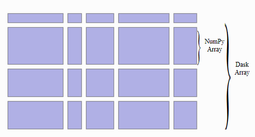
Dask.array: A multidimensional array composed of many small NumPy arrays.
import dask.array as da
x = da.random.random((10000, 10000), chunks=(1000, 1000))
x
This creates a random Dask Array of dimensions 10000 by 10000. The chunks argument allows you to define how the Array can be broken up. In this case, the array can be broken up in ten pieces, with each piece by dimensions 1000 by 1000. Using the right chunk size will become extremely important in helping you optimize advanced algorithms.
More on chunks here: https://docs.dask.org/en/latest/array-chunks.html
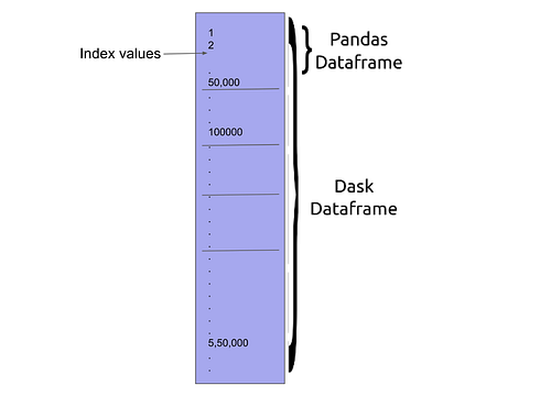
Dask.DataFrame: Similarly to a dask array, a Dask DataFrame is a logical connection of many Pandas DataFrames (ex: using many hard drives to connect different datasets)
from dask import datasets
import dask.dataframe as dd
df = datasets.timeseries()
You will notice that if you try to see the DataFrame by calling it directly with its variable, you will not be able to see any data.
dfThis is because Dask is inherently lazy, meaning it will not compute anything unless you explicitly tell it to do so. Calling persist() will save it to your computer’s memory (RAM) so you can see the data directly. Make sure that your computer has enough RAM for you to do so!
df.persist()
df
I always like to refer to the original source of documentation which provides the most accurate information, so I highly suggest exploring the Dask page to learn more about Dask DataFrames and Arrays.
Visualizing task graphs
Task graphs are very useful to help you understand how dask is parallelizing the tasks in the backgrounds and debug to understand how certain tasks can be parallelized while others cannot.
There two ways you can visualize task graphs.
- You can visualize it by saving the task graph as an image locally. This is used for simpler computations to see how Dask divides the tasks to compute the tasks in parallel.
import dask.array as da
x = da.ones((50, 50), chunks=(5, 5))

y = x + x.T

# y.compute()
y.visualize(filename='transpose.svg')- You can use the dask dashboard to visualize an interactive task graph (available by default at localhost:8787). This is used to visualize more complicated computations that take a long time to finish.
Conclusion
This was a short article showcasing how Dask works. I hope I explained it well! Feel free to leave any feedback on my explanations! Thank you for reading :)