Mini-Batch Gradient Descent

Mini-batch gradient descent. In large-scale applications (such as the ILSVRC challenge), the training data can have on order of millions of examples. Hence, it seems wasteful to compute the full loss function over the entire training set in order to perform only a single parameter update. A very common approach to addressing this challenge is to compute the gradient over batches of the training data. For example, in current state of the art ConvNets, a typical batch contains 256 examples from the entire training set of 1.2 million. This batch is then used to perform a parameter update:

# Vanilla Minibatch Gradient Descent
while True:
  data_batch = sample_training_data(data, 256) # sample 256 examples
  weights_grad = evaluate_gradient(loss_fun, data_batch, weights)
  weights += - step_size * weights_grad # perform parameter update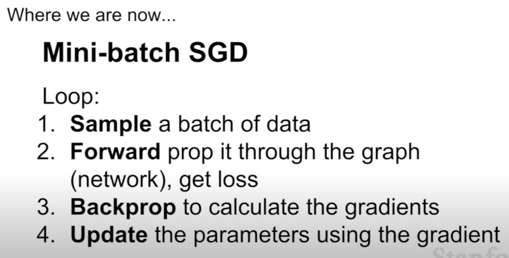

The reason this works well is that the examples in the training data are correlated. To see this, consider the extreme case where all 1.2 million images in ILSVRC are in fact made up of exact duplicates of only 1000 unique images (one for each class, or in other words 1200 identical copies of each image). Then it is clear that the gradients we would compute for all 1200 identical copies would all be the same, and when we average the data loss over all 1.2 million images we would get the exact same loss as if we only evaluated on a small subset of 1000. In practice of course, the dataset would not contain duplicate images, the gradient from a mini-batch is a good approximation of the gradient of the full objective. Therefore, much faster convergence can be achieved in practice by evaluating the mini-batch gradients to perform more frequent parameter updates.