Gradient Descent

Gradient descent is an optimization algorithm commonly used to train machine learning models and neural networks.

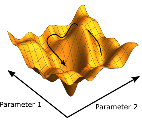
See Parameter Landscape and familiarize yourself with Partial Derivatives first.

Let $J(\theta )$ be a differentiable function of the parameter vector $\theta$. Define the gradient of $J(\theta )$ as: ${\nabla }_{\theta }J(\theta )=\left(\frac{\partial J(\theta )}{\partial {\theta }_1}⋮\cdots ⋮\frac{\partial J(\theta )}{\partial {\theta }_n}\right)$

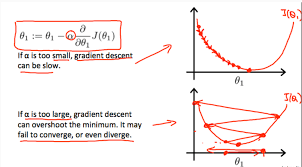
To find a local minimum of $J(\theta )$, update $\theta$ in the direction of the negative gradient:

$$\theta :=\theta -\alpha {\nabla }_{\theta }J(\theta )$$

where:

• $\alpha$ is the learning rate (step-size parameter)

Intuition

The gradient points uphill; you step in the opposite direction. The learning rate is how far you trust that local direction. Too big and you overshoot past the valley floor; too small and you crawl. Everything fancy (momentum, Adam, schedules) is just a better way to answer “how much should I trust this gradient right now?”

while True:
  weights_grad = evaluate_gradient(loss_fun, data, weights)
  weights += - step_size * weights_grad # perform parameter update

There are two ways to compute the gradient:

• Numerical Gradient: not practically feasible, see page for code
• Analytical Gradient: uses calculus

Now, Backpropagation comes into the picture when we look at how to compute the evaluate_gradient function. For SVM for example, we have a fixed analytical gradient that we calculated, but we want to be able to do this for any function.

Challenges:

• Running into a local minimum or saddle point, fixed by adding stochasticity

Aside: WAIT, Serendipity, we saw this sort of idea in E&M with Electric Potential Energy, remember the lab. We saw that the gradient represents the change in potential (wait how do Electric Field, Electric Potential, and Electric Potential Energy relate?)

Optimizer

SGD:

momentum update

# Vanilla Gradient Descent
x += - learning_rate * dx
 
# Momentum update
"""
- We build up velocity along shallow directions.
- Velocity becomes damped in steep direction due to quickly changing sign.(you can initialize v=0)
- Intuition: a ball rolling down the loss surface. In a narrow ravine, raw
  gradients ping-pong across the walls; momentum averages them out so the
  ball keeps moving along the valley floor.
"""
v = mu * v - learning_rate * dx # mu * v is like the friction, mu is a hyperparameter, mu = 0.5 or 0.9
x += v
 
# Nesterov Momentum update (this is a trick to get a look-ahead)
v_prev= v
v = mu * v - learning_rate * dx
x += -mu * v_prev + (1 + mu) * v
 
# Adagrad (per-parameter learning rate: params that have seen big
# gradients get smaller steps, so each dimension progresses at a
# similar pace. Downside: cache grows forever, eventually stalling.)
cache += dx ** 2
x += - learning_rate * dx / (np.sqrt(cache) + 1e-7)
 
# RMSProp (Adagrad with a leaky cache: recent gradients count more,
# old ones decay away, so progress doesn't grind to a halt.)
cache += decay_rate * cache + (1-decay_rate) * dx ** 2
x += - learning_rate * dx / (np.sqrt(cache) + 1e-7)
 
# Adam (momentum + RMSProp: remember the average direction AND the
# per-parameter magnitude. First moment m = "where am I going", second
# moment v = "how noisy is this direction".)
m = beta1*m + (1-beta1)*dx # update first moment
v = beta2*v + (1-beta2)*(dx**2) # update second moment
m /= 1 - beta1**t # correct bias (only relevant in the first few iterations)
v /= 1 - beta2**t # ""
x += - learning_rate * m / (np.sqrt(v) + 1e-7)

As you scale up your network, it looks more like a bowl. Local minimum become less and less of an issue. It only really happens with small networks. - Andrej Karpathy

Adam is the default choice. Adam with ${\beta }_1=0.9$, ${\beta }_2=0.999$, $\text{lr}=10^{-3}$ or $5\times 10^{-4}$ is a great starting point for many models. See original paper.

The bias correction (m /= 1 - beta1**t and similarly for $v$) matters because both moments are initialized at zero. Without correction, the first few steps would be biased toward zero and the effective step would be tiny.

AdamW: decoupled weight decay

Standard Adam folds the L2 penalty into the gradient (dx = compute_gradient(x) + wd * x), which then gets scaled by the per-parameter 1/sqrt(second_moment) factor, so large-gradient parameters get less regularization than small-gradient ones. AdamW instead applies the decay term after the moment-scaled update: $x_{t+1}=x_t-\alpha \cdot {\hat{m}}_t/(\sqrt{{\hat{v}}_t}+\epsilon )-\alpha \cdot \text{wd}\cdot x_t$ This restores the original “shrink toward zero” behavior. Empirically AdamW > Adam+L2 on ImageNet and most modern transformer training. See Weight Decay.

Learning rate schedules

Every optimizer above (SGD, SGD+Momentum, RMSProp, Adam, AdamW) has the learning rate as a hyperparameter. Common decay schedules:

• Step: drop LR by 0.1× at fixed epochs (e.g. ResNet: epochs 30, 60, 90)
• Cosine: ${\alpha }_t=\frac{1}{2}{\alpha }_0(1+\cos (t\pi /T))$
• Linear: ${\alpha }_t={\alpha }_0(1-t/T)$
• Inverse sqrt: ${\alpha }_t={\alpha }_0/\sqrt{t}$ (Vaswani Transformer)
• Linear warmup: ramp LR from 0 over the first ~5000 iterations to prevent loss explosion at high initial LRs

Empirical rule of thumb: if you increase batch size by $N$, scale the initial LR by $N$ (Goyal et al., “Accurate, Large Minibatch SGD: Training ImageNet in 1 Hour”).

First- vs second-order optimization

All of the above are first-order: they use only the gradient (linear approximation) and step to minimize that approximation. Second-order methods (Newton, L-BFGS) use gradient + Hessian to form a quadratic approximation and step to its minimum. Quadratic approximation fits the curvature better, so in principle takes fewer steps, but storing/inverting the $d\times d$ Hessian is infeasible when $d$ is millions of parameters, which is why deep learning lives on first-order methods.

Picture: a first-order method only knows the slope under its feet, so it takes a fixed-size step downhill. A second-order method also knows how fast the slope itself is changing, and picks a step that lands near the bottom of a local bowl in one shot.

From CS231n Lec 3 slides 49-92 (gradient descent, SGD problems, SGD+Momentum, RMSProp, Adam, AdamW, learning rate schedules, first/second-order).

Related

• Mini-Batch Gradient Descent
• Stochastic Gradient Descent

Gradient Descent from first principles

I thought I understood gradient descent, but it’s very easy to forget the underlying motivations. Like sure, you can just say that you make a gradient update in the direction.

My understanding is mainly written in Backpropagation, but rewriting some ideas as a refresher here.

Say we want to estimate parameters for a linear model $\hat{y}=ax+b$:

• We want parameters $a,b$ that best fit an input set of $(x_i,y_i)$ values
• You can do this easily with Linear Regression, but let’s be fancy and use gradient descent

We define our loss as the squared error: $L=(y-\hat{y}{)}^2$

where:

• $\hat{y}$ is our estimated value
• $y$ are measurements

What happens with y?

Remember we are taking partial derivatives. $y$ and $\hat{y}$ are both variables. We keep the parameters fixed and play around with various $y$ values

We update parameters $a,b$ based on the gradient to minimize the loss: $a\leftarrow a+\alpha \cdot \frac{\delta L}{\delta a}$ $b\leftarrow b+\alpha \cdot \frac{\delta L}{\delta b}$

where:

• $\alpha$ is the learning rate

So we have the following two functions:

• $L=(y-\hat{y}{)}^2$
• $\hat{y}=ax+b$

We apply the chain rule to compute the partial derivatives: $\frac{\delta L}{\delta a}=\frac{\delta L}{\delta \hat{y}}\frac{\delta \hat{y}}{\delta a}=(2(y-\hat{y})\cdot (-1))\cdot (x)=-2(y-(ax+b))\cdot x$ $\frac{\delta L}{\delta b}=\frac{\delta L}{\delta \hat{y}}\frac{\delta \hat{y}}{\delta b}=(2(y-\hat{y})\cdot (-1))\cdot (1)=-2(y-(ax+b))$

If you’re not sure how I got this, revisit your partial derivatives. Usually updates are done in small batches, but for simplicity assume we read in a single value before each update.

Wait, do we care about \frac{\delta L}{\delta a} or \frac{\delta a}{\delta L}?

$\frac{\delta a}{\delta L}$ doesn’t really make sense. We want to find a parameter $a$ such that $L$ has a minimum.

It’s like having a function $y=x^2$. What is $\frac{dx}{dy}$? Just the inverse, but not useful to us. We care about $\frac{dy}{dx}$ because that tells us how $y$ changes as we change $x$, not how $x$ changes as we change $y$ (since $y$ is the output, we can’t modify it directly)

If you did a gradient update of $a$ with $\frac{\delta a}{\delta L}$, you’d get incorrect results: that tells how $a$ changes as you change $L$, but we want to see how $L$ changes as you change $a$

I was having trouble visualizing gradient descent updates. Like if you plot your function, and observations are just points, you’re actually looking at different gradient points:

• Remember that the set of parameters represent the entire function, not a particular point
• With gradient descent, if you sample a wide enough variety of points, as you update your gradients you get closer and closer to points that represent the function

I’m having trouble visualizing this. Ahh actually I can see it