Gradient

Numerical Gradient

The numerical gradient is based off the definition of the derivative: $f^{\prime }(x)={\lim }_{h\to 0}\frac{f(x+h)-f(x)}{h}$

However, the numerical gradient is slow to compute, because you need to iterate over every single dimension. However, it is quite accurate, so you can use it to check the correctness your Analytical Gradient. This is called a gradient check.

h = 0.0001
 
a = 2.0
b = -3.0
c = 10.0
 
d1 = a*b +c
c += h
d2 = a*b +c
 
print("slope", (d2-d1)/h)

We compute the numerical gradient with respect to some weight $W$, by changing the values of $W$ dimension by dimension, and see how the loss changes:

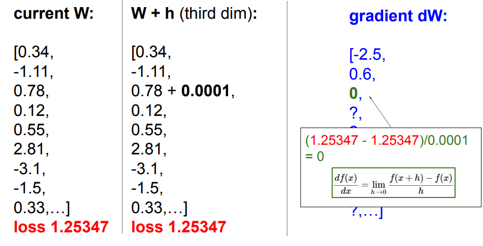
We update the weights in the direction that minimizes the Loss Function.

In practice, we might want to use the centered difference formula which often works better: $f^{\prime }(x)={\lim }_{h\to 0}\frac{f(x+h)-f(x-h)}{2h}$

Computing the gradient numerically with finite differences

Below is a generic function that takes a function f, a vector x to evaluate the gradient on, and returns the gradient of f at x:

def eval_numerical_gradient(f, x):
  """
  a naive implementation of numerical gradient of f at x
  - f should be a function that takes a single argument
  - x is the point (numpy array) to evaluate the gradient at
  """
 
  fx = f(x) # evaluate function value at original point
  grad = np.zeros(x.shape)
  h = 0.00001
 
  # iterate over all indexes in x
  it = np.nditer(x, flags=['multi_index'], op_flags=['readwrite'])
  while not it.finished:
 
    # evaluate function at x+h
    ix = it.multi_index
    old_value = x[ix]
    x[ix] = old_value + h # increment by h
    fxh = f(x) # evalute f(x + h)
    x[ix] = old_value # restore to previous value (very important!)
 
    # compute the partial derivative
    grad[ix] = (fxh - fx) / h # the slope
    it.iternext() # step to next dimension
 
  return grad

Following the gradient formula we gave above, the code above iterates over all dimensions one by one, makes a small change h along that dimension and calculates the partial derivative of the loss function along that dimension by seeing how much the function changed. The variable grad holds the full gradient in the end.

Practical considerations. Note that in the mathematical formulation the gradient is defined in the limit as h goes towards zero, but in practice it is often sufficient to use a very small value (such as 1e-5 as seen in the example). Ideally, you want to use the smallest step size that does not lead to numerical issues. Additionally, in practice it often works better to compute the numeric gradient using the centered difference formula: [f(x+h)−f(x−h)]/2h[f(x+h)−f(x−h)]/2h . See wiki for details.

We can use the function given above to compute the gradient at any point and for any function. Lets compute the gradient for the CIFAR-10 loss function at some random point in the weight space:

# to use the generic code above we want a function that takes a single argument
# (the weights in our case) so we close over X_train and Y_train
def CIFAR10_loss_fun(W):
  return L(X_train, Y_train, W)
 
W = np.random.rand(10, 3073) * 0.001 # random weight vector
df = eval_numerical_gradient(CIFAR10_loss_fun, W) # get the gradient

The gradient tells us the slope of the loss function along every dimension, which we can use to make an update:

loss_original = CIFAR10_loss_fun(W) # the original loss
print 'original loss: %f' % (loss_original, )
 
# lets see the effect of multiple step sizes
for step_size_log in [-10, -9, -8, -7, -6, -5,-4,-3,-2,-1]:
  step_size = 10 ** step_size_log
  W_new = W - step_size * df # new position in the weight space
  loss_new = CIFAR10_loss_fun(W_new)
  print 'for step size %f new loss: %f' % (step_size, loss_new)
 
# prints:
# original loss: 2.200718
# for step size 1.000000e-10 new loss: 2.200652
# for step size 1.000000e-09 new loss: 2.200057
# for step size 1.000000e-08 new loss: 2.194116
# for step size 1.000000e-07 new loss: 2.135493
# for step size 1.000000e-06 new loss: 1.647802
# for step size 1.000000e-05 new loss: 2.844355
# for step size 1.000000e-04 new loss: 25.558142
# for step size 1.000000e-03 new loss: 254.086573
# for step size 1.000000e-02 new loss: 2539.370888
# for step size 1.000000e-01 new loss: 25392.214036

Update in negative gradient direction. In the code above, notice that to compute W_new we are making an update in the negative direction of the gradient df since we wish our loss function to decrease, not increase.

Effect of step size. The gradient tells us the direction in which the function has the steepest rate of increase, but it does not tell us how far along this direction we should step. As we will see later in the course, choosing the step size (also called the learning rate) will become one of the most important (and most headache-inducing) hyperparameter settings in training a neural network. In our blindfolded hill-descent analogy, we feel the hill below our feet sloping in some direction, but the step length we should take is uncertain. If we shuffle our feet carefully we can expect to make consistent but very small progress (this corresponds to having a small step size). Conversely, we can choose to make a large, confident step in an attempt to descend faster, but this may not pay off. As you can see in the code example above, at some point taking a bigger step gives a higher loss as we “overstep”.

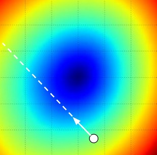
Visualizing the effect of step size. We start at some particular spot W and evaluate the gradient (or rather its negative - the white arrow) which tells us the direction of the steepest decrease in the loss function. Small steps are likely to lead to consistent but slow progress. Large steps can lead to better progress but are more risky. Note that eventually, for a large step size we will overshoot and make the loss worse. The step size (or as we will later call it - the learning rate) will become one of the most important hyperparameters that we will have to carefully tune.

A problem of efficiency. You may have noticed that evaluating the numerical gradient has complexity linear in the number of parameters. In our example we had 30730 parameters in total and therefore had to perform 30,731 evaluations of the loss function to evaluate the gradient and to perform only a single parameter update. This problem only gets worse, since modern Neural Networks can easily have tens of millions of parameters. Clearly, this strategy is not scalable and we need something better.

Related

• Finite Differences