The Dataset

The dataset we are using to learn to program our first Artificial Neural Network is available here, as a .csv file, describing the current bank situations, and we are trying to predict whether these customers are going to exit the bank within the next 6 months.

The 5 steps to building a Neural Network

If you read the last article I told you to read, then you remember the 5 steps I told you to program an ANN, which is the following:

1. Import the training set which serves as the input layer.
2. Forward propagate the data from the input layer through the hidden layer to the output layer, where we get a predicted value y. Forward propagation is the process by which we multiply the input node by a random weight, and applying the activation function.
3. Measure the error between the predicted value and the real value.
4. Backpropagate the error and use gradient descent to modify the weights of the connections.
5. Repeats these steps until the error is minimized sufficiently.

However, when it comes to coding the Artificial Neural Network, since we are using libraries to help us, specifically the Keras library, our lines of code will be dramatically reduced, but we will need to include a few additional steps. This new process will be summarized in 5–6 steps.

Step 1: Process the data and split into a training and test set
Step 2: Build the Artificial Neural Network Structure
Step 3: Train the Artificial Neural Network
Step 4: Use the model to predict!
Step 5(Optional): Tune the model for better accuracy

Step 1: Process the data and split into a training and test set

Before we actually build our exciting ANN, we need to first process our data. Oftentimes, data preprocessing is the most complicated part of the process. Building the algorithm itself is pretty easy once you get the hang of it, but every time you want to build a model with a new type of dataset, you will probably run into data processing problems, which might take a lot of time to understand and think of ways to process them.

Lines 1–4: Import the data. We are using pandas to do so, in line 4, where we import the .csv file and specify the file location. Take a moment to look at how the dataset is structured.

Our Dataset

Lines 5–6: Separate into X(input values) and Y(output values, i.e. the value we want to predict), transforming the original Dataframe into arrays. Notice we only take the values at the columns 3 to 13, since those are the values which are going to affect the output. The “number”, “customerID”, and “Surname” are not going to affect the output, hence we do not consider it in our input.

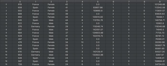
Our inputs(X). Each row represents a customer, while each column represents a feature of the customer, such as Gender and Geography.

Our target values(y)

Lines 9–19: Making the code understandable by the machine by transforming it into numbers (encoding categorical data into numerical data). If you look carefully at the dataset, you can see that there are two categorical types of data. “Gender” and “Geography”. Each of these types of values returns strings, which the computer cannot process. Hence, we need to first encode it into numbers. We use the LabelEncoder and OneHotEncoder function to do that. For “Gender”, there are 2 categories, “Male” and “Female”, hence we can transform that into the integers 0 and 1. For “Geography”, there are 3 types: “Germany”, “France”, and “Spain”, which are transformed into 0,1 and 2. However, there is also this thing called a dummy variable that you need to remove.

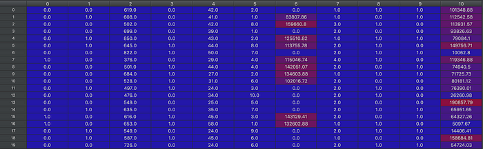
Now, X is only composed of numbers.

Lines 22–23: Splitting the data we have into a training set and test set. This is extremely important because we need to verify the accuracy of the model after we are done training it and see how well it will perform with data that it has not trained on. This is where the test set comes in. We use the sci-kit learn library to do this. Test_size = 0.2 means that 20% of the dataset will be used for testing, and the other 80% will be used for training. Random_state = 0 is a parameter that basically makes each randomization constant, so no matter how many times you split the dataset, it will split the same way.

Lines 26–29: The final step of the data preprocessing is to apply feature scaling (also known as data normalization) on the dataset. This means that we will transform the values to fit between -1and 1. If we look at X_train or X_test again, we will see how it works.

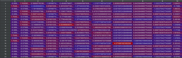
A look at X_train

Step 2: Build the Artificial Neural Network Structure

Now that we are done with the data preprocessing part, we are finally ready to create the structure of our Artificial Neural Network. As we know, an Artificial Neural Network is composed of 3 types of layers: the input layer, the hidden layer, and the output layer.

1. Initialize the Neural Network using the Sequential() call to “classifier”, which will be the name of our model, since the one we are going to build is a classifier, i.e. the output it will return is an integer value, 0 or 1.

2. Define the input layer and first hidden layer. Add Dropout regularization, which prevents overfitting.

Let’s clearly look at the parameters we are adding.

input_dim = 11: This specifies the dimensions of our input (i.e. how many types of inputs do we have)

Units = 6: This is how many units (Neurons) our connected layer (the hidden layer attached) is going to have.

kernel_initializer = ‘uniform’: The term kernel_initializer is a fancy term for which statistical distribution or function to use for initializing the weights. You don’t need to worry too much about that.

activation = ‘relu’: This input parameter specifies the type of activation function that we are going to use, which is the reLU (rectifier linear unit) activation function in our case. Although it is two linear pieces, it has been proven to work well in neural networks. This Medium article explains it very well.

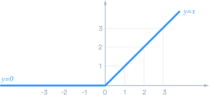
ReLU Activation Function (credit)

3. Defining the second hidden layer. We already defined how many Neurons this hidden layer is going to have (6), hence we don’t need to specify its input_dim again. We once again have the Dropout regularization function.
4. Defining our output layer. Notice that units = 1, because for our output, we want it to return a single integer value, either 0 or 1.
5. Finally, compile the Neural Network.

Explanation of the Input parameters for compile function
optimizer = ‘adam’: This is the optimizer we are going to use. It is the way the machine will do Gradient Descent. The optimizer controls the learning rate throughout training, i.e. how fast the optimal weights for the model are calculated. A smaller learning rate may lead to more accurate weights (up to a certain point), but the time it takes to compute the weights will be longer. Adam is generally a good optimizer to use for many cases.

loss = ‘binary_crossentropy’; this defines how we get closer to our loss. In our case, since our output is binary, we use ‘binary_crossentropy’.

metrics = [‘accuracy’]: This is how we measure how accurate our Neural Netowrk will be during the training phase. Since our output is binary, we use the ‘accuracy’ parameter.

Step 3: Train the Artificial Neural Network

This step is a simple line where we define the data we are going to use to fit. We stored our input and output values in X_train and y_train.

The batch size defines the number of samples that will be propagated through the network.

For instance, let’s say you have 1050 training samples and you want to set up a batch_size equal to 100. The algorithm takes the first 100 samples (from 1st to 100th) from the training dataset and trains the network.

• one epoch = one forward pass and one backward pass of all the training examples
• batch size = the number of training examples in one forward/backward pass. The higher the batch size, the more memory space you’ll need.
• number of iterations = number of passes, each pass using [batch size] number of examples. To be clear, one pass = one forward pass + one backward pass (we do not count the forward pass and backward pass as two different passes).

Ex: if you have 1000 training examples, and your batch size is 500, then it will take 2 iterations to complete 1 epoch.

Once you start running that code, you can sit back, take a nap, watch some Netflix, and wait for your computer to do the magic. After you are done, you should get an accuracy of around 85%!!

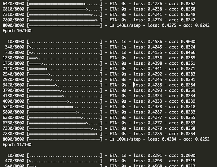
What it should look like while you are training your model.

Step 4: Use the model to predict!

Now that our model has finished training, we can measure the real accuracy of our model by testing it on an unknown dataset. We do this with the .predict method. The classifier predicts a set of values, stored in y_pred. In line 3, we round the value of y_pred to either 0 or 1. Finally, we use the Confusion Matrix to see how many values we got right or wrong.

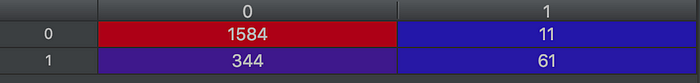
What our confusion Matrix shows (click here to read more about how a confusion matrix works)