Decision Tree

A decision tree is a hierarchical classifier (or regressor) built by recursively splitting the feature space on one variable at a time.

• Simple, interpretable, but high-variance
• Often combined via Bagging or Boosting for better performance

Building a Tree

1. Start with one node (the root) containing all data
2. Recursively split each leaf: choose a variable $j$ and threshold $t$, partition points into $S_L=\{(x_i,y_i):x_{ij}\le t\}$ and $S_R=\{(x_i,y_i):x_{ij}>t\}$
3. Stop based on some criterion (see below)
4. Predict by walking down the tree from root to leaf and returning the leaf’s majority label (classification) or mean label (regression)

Which Split?

Choose a node loss $\ell (S)$ that is small for pure nodes (all same label) and large for mixed ones. Pick the split that minimizes the weighted sum of child node costs.

$(j^{\ast },t^{\ast })=\arg {\min }_{j,t}|S_L|\cdot \ell (S_L)+|S_R|\cdot \ell (S_R)$

where:

• $S_L,S_R$ are the left/right partitions at threshold $t$ on feature $j$
• $\ell (S)$ is the node loss measuring impurity

Intuition

Each split is a yes/no question. You want the question that carves the data into the cleanest piles: ideally “all cancer” on one side, “all healthy” on the other. The weighted sum is there because a tiny-but-pure child shouldn’t outvote a large mixed one. Big children matter more.

For each feature $j$, you only need to try $\le n$ thresholds (between sorted values of $x_{ij}$).

Node Loss Functions (Classification)

Let ${\hat{p}}_c=\frac{1}{|S|}{\sum }_{i\in S}1[y_i=c]$ be the fraction of class $c$ in node $S$, and $\hat{y}=\arg {\max }_c{\hat{p}}_c$.

• Misclassification loss: $\ell (S)=1-{\hat{p}}_{\hat{y}}$ (fraction you’d get wrong if you guessed the majority)
• Entropy: $\ell (S)=-{\sum }_c{\hat{p}}_c\log {\hat{p}}_c$ (this is Shannon entropy)
• Gini index: $\ell (S)={\sum }_c{\hat{p}}_c(1-{\hat{p}}_c)$ (probability two random draws from the node disagree)

Intuition

Entropy is how surprised you’d be by a random label drawn from this node. A pure node, no surprise. A 50/50 node, maximum surprise. Splitting to reduce entropy = asking the most informative question next. Gini is almost the same idea with a different curve: the chance that two people picked at random from this node would disagree on the label. Misclassification loss is flat in the middle, so it can’t tell a 60/40 split apart from a 51/49 one; entropy and Gini curve more, so gradients flow and splits get chosen more sensibly.

Entropy and Gini are differentiable and tend to produce more balanced splits than misclassification.

Regression loss: $\ell (S)=\frac{1}{|S|}{\sum }_{i\in S}(y_i-{\bar{y}}_S{)}^2$, where ${\bar{y}}_S$ is the mean label in $S$.

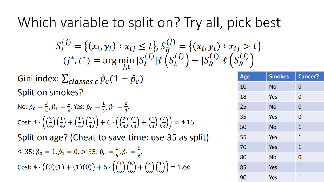
Example: Gini Split

Age	Smokes	Cancer?
10	No	0
18	Yes	0
25	No	0
35	Yes	0
50	No	1
55	Yes	1
70	Yes	1
80	No	0
85	Yes	1
90	Yes	1

Split on smokes? No (4 pts): ${\hat{p}}_0=3/4,{\hat{p}}_1=1/4$. Yes (6 pts): ${\hat{p}}_0=1/3,{\hat{p}}_1=2/3$. Weighted Gini cost: $4\cdot (3/4\cdot 1/4+1/4\cdot 3/4)+6\cdot (1/3\cdot 2/3+2/3\cdot 1/3)=4.16$

Split on age > 35? $\le 35$ (4 pts): all 0. $>35$ (6 pts): ${\hat{p}}_0=1/6,{\hat{p}}_1=5/6$. Cost: $4\cdot 0+6\cdot (1/6\cdot 5/6+5/6\cdot 1/6)=1.66$ → age wins.

Stopping Criteria

• Max depth reached
• Few examples in a leaf (e.g., $\le 5$)
• Leaf is homogeneous (pure)
• Split improvement $\Delta =|S|\ell (S)-(|S_L|\ell (S_L)+|S_R|\ell (S_R))$ is below a threshold
• Running time budget exhausted

Pruning

Alternative to early stopping: grow the tree fully, then prune. Choose the subtree that minimizes

${\sum }_{\text{leaves }v}\text{error}(v)+\alpha \cdot (\text{number of leaves})$

where:

• $\alpha$ controls the tradeoff: $\alpha =0$ keeps the full tree, $\alpha \to \infty$ collapses to a single node

Growing first then pruning lets the tree see useful splits that only pay off a few levels down, which a greedy early-stop would miss. Pick $\alpha$ via validation.

A decision stump is a 3-node tree (one split). Very weak on its own but useful as the base learner in AdaBoost.

Pros / Cons

• Interpretable, easy to visualize
• Handles mixed feature types, no need to normalize
• Can model nonlinear (axis-aligned) boundaries
• High variance: small data changes produce very different trees
• Struggles with boundaries that are not axis-aligned (e.g. a diagonal line)
• Tends to overfit without regularization/pruning

Improvements:

• Bootstrap Aggregating (Bagging): average many trees on bootstrap samples
• Random Forest: bagging + random feature subsets at each split
• Boosting (AdaBoost, Gradient Boosted Trees)

Slides: http://www.gautamkamath.com/courses/CS480-fa2025-files/lec7.pdf

Related

• Entropy
• Random Forest
• Gradient Boosted Decision Tree