Neural Network

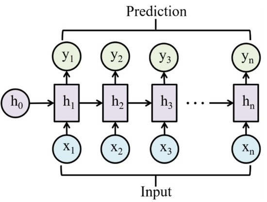
Recurrent Neural Network (RNN)

An RNN is a neural network that processes sequences by maintaining a hidden state updated at each timestep, “learning from the past”.

Good for time series data.

Resources

• https://karpathy.github.io/2015/05/21/rnn-effectiveness/
• https://www.youtube.com/watch?v=TQQlZhbC5ps&ab_channel=CodeEmporium
• https://cs231n.github.io/rnn/
• https://www.deeplearningbook.org/contents/rnn.html

Three types of models:

• Vector-Sequence: e.g. captioning an image
• Sequence-Vector: e.g. sentiment analysis, converting a sentence into a number
• Sequence-Sequence: e.g. language translation

Disadvantages

• Slow to train
• Long sequences lead to Vanishing Gradient / Exploding Gradients, solved by Long Short-Term Memory

Output $y_t$ vs hidden state $h_t$

Had this confused when I was reading the World Models paper. In an RNN, the hidden state is the internal representation that carries information forward in time, designed to be rich enough to summarize the relevant history.

In my words

You can think of $h_t$ (the hidden state) as sitting right before some transformation $W$ to get the output $y_t$ ($y_t=W{h}_t$). But $h_t$ is propagated through time. It doesn’t make sense to propagate $y_t$, which is generally lossier than the hidden state

The output $y_t$ is typically computed as a simple transformation of $h_t$:

$$y_t=W{h}_t+b$$

or through a softmax layer for classification.

Propagating $y_t$ instead of $h_t$ wouldn’t make sense because $y_t$ is usually a lower-dimensional, task-specific (and often lossy) projection of $h_t$. It doesn’t preserve enough information for the next step to condition on.

That’s why the recurrence is defined in terms of $h_t$:

$$h_t=f(h_{t-1},x_t)$$

Sequence patterns (CS231n Lec 7)

A vanilla feedforward net is one-to-one (fixed-size input → fixed-size output). RNNs unlock four other patterns by treating either the input, the output, or both as a sequence:

Pattern	Example	Shape
one-to-many	image captioning (image → sentence)	1 input → $T$ outputs
many-to-one	video action recognition / sentiment	$T$ inputs → 1 output
many-to-many (aligned)	per-frame video classification	$T$ inputs → $T$ outputs
many-to-many (seq2seq)	machine translation	$T$ inputs → $T^{\prime }$ outputs

Key idea: RNNs maintain an internal state that’s updated as the sequence is processed. The same function $f_W$ and the same parameters $W$ are used at every timestep (hence “recurrent”).

Vanilla (Elman) RNN

$h_t=\tanh (W_{hh}{h}_{t-1}+W_{xh}{x}_t),y_t=W_{hy}{h}_t$

Same $W_{hh},W_{xh},W_{hy}$ at every timestep. Equivalently in stacked form: $h_t=\tanh \left(W\right[\begin{array}{c}{h}_{t-1}\\ x_t\end{array}\left]\right)$ where $W=[W_{hh}{W}_{hx}]$.

Intuition

A CNN shares weights across space; an RNN shares them across time. The same function $f_W$ fires at every step, reading the current input plus a running summary of everything seen so far, and writing back an updated summary. The hidden state is that running summary, compressed into a fixed-size vector no matter how long the sequence.

Computational graph & weight sharing

Unrolling the recurrence gives a chain $h_0\to h_1\to h_2\to \cdots \to h_T$, with the same $W$ feeding every cell.

• Many-to-many loss: sum per-step losses $L={\sum }_t{L}_t$
• Many-to-one: only the final $h_T$ feeds the output
• One-to-many with a single input: $x$ is fed at $t=1$ and either zeros or the previous output $y_{t-1}$ is fed at later steps

Character-level language model example

Vocabulary [h, e, l, o], training sequence “hello”. Each character is a one-hot input; output at each step is the softmax distribution over the next character. Train with cross-entropy on (h→e, e→l, l→l, l→o).

Sampling at test time: feed a seed character, sample from the softmax, feed the sample back as the next input. Repeat. This is how Karpathy’s min-char-rnn.py (112 lines of NumPy) generates Shakespeare, Linux source code, or LaTeX algebraic geometry papers after training on each corpus.

Embedding trick: matrix-multiplying $W_{xh}$ by a one-hot vector just selects the corresponding column. So in practice we factor $W_{xh}$ into a separate embedding layer that maps each token id to a learned dense vector.

Backpropagation through time (BPTT)

Forward through the entire sequence to compute the loss, then backward through the entire sequence to compute gradients.

Infeasible for long sequences

For something like all of Wikipedia, you’d hold $T$ hidden states in memory and backprop through all of them

Truncated BPTT: carry hidden states forward in time forever, but only backprop through chunks of $\sim 100$ timesteps. Run forward+backward on chunk 1, carry the final hidden state into chunk 2, run forward+backward on chunk 2, etc. Loses long-range gradient signal but is the only way to train on very long sequences.

Vanilla RNN gradient flow & vanishing/exploding

Backprop from $h_t$ to $h_{t-1}$ goes through $\tanh$ then multiplies by $W_{hh}^{\top }$: $\frac{\partial h_t}{\partial h_{t-1}}={\tanh }^{\prime }(W_{hh}{h}_{t-1}+W_{xh}{x}_t)W_{hh}$

The gradient w.r.t. $W$ from a loss at step $T$ chains $T-1$ of these factors: $\frac{\partial L_T}{\partial W}=\frac{\partial L_T}{\partial h_T}\left({\prod }_{t=2}^T\frac{\partial h_t}{\partial h_{t-1}}\right)\frac{\partial h_1}{\partial W}=\frac{\partial L_T}{\partial h_T}({\prod }_{t=2}^T{\tanh }^{\prime }(\cdot )W_{hh})\frac{\partial h_1}{\partial W}$

Two failure modes (controlled by largest singular value of $W_{hh}$):

• Largest singular value > 1 → exploding gradients. Fix: gradient clipping (if grad_norm > thresh: grad *= thresh/grad_norm)
• Largest singular value < 1 → vanishing gradients (and ${\tanh }^{\prime }<1$ makes it worse). Fix: switch to LSTM / GRU, whose additive cell-state path gives gradient an uninterrupted highway

Intuition: multiplying by $W_{hh}$ fifty times is like compounding interest. If the dominant eigenvalue is 0.9, a signal fifty steps back shrinks to $0.9^{50}\approx 0.005$; if it’s 1.1, it blows up to 117. There’s almost no knife-edge where it stays useful, which is why LSTMs replace repeated multiplication with an additive path.

Multilayer (deep) RNNs

Stack RNN layers along a depth axis: each layer receives the lower layer’s hidden state as its input. 2–4 layers is typical; deeper than that is rare for plain RNNs.

Searching for interpretable cells

Karpathy/Johnson/Fei-Fei (2015) trained a char-RNN on text and visualized individual hidden-state coordinates. Some cells turn out to fire on interpretable patterns: a quote-detection cell (on inside "…"), a line-length tracker, an if-statement cell, a comment-block cell, a code-depth cell. Most cells are uninterpretable, but the existence of any structured ones is a small surprise given there’s no architectural pressure for it.

RNN tradeoffs

Pros:

• Can process inputs of any length, model size doesn’t grow with input length
• Same weights at every timestep, symmetric processing
• In theory, step $t$ can use info from arbitrarily far back

Cons:

• Recurrent computation is sequential, can’t parallelize across time
• In practice, hard to access info from many steps back (vanishing gradient)

These limitations are exactly what motivated attention and Transformers (see Lec 8).

From CS231n 2024 Lec 7 slides 21-107 (sequence patterns, vanilla RNN, computational graphs, char-level LM, BPTT/truncated BPTT, multilayer RNNs, vanilla gradient flow, vanishing/exploding gradients, gradient clipping, interpretable cells, RNN tradeoffs). Note: 2026 Lec 7 PDF not yet published, content cited from 2024 deck (same topic as the 2026 syllabus).

Recurrent Convolutional Network for video (CS231n 2025 Lec 10)

For video, we want a recurrent net whose hidden state is a spatial feature map not a vector. Vanilla RNN at each step:

$h_{t+1}=\tanh (W_h{h}_{t-1}+W_x{x}_t)$

In a Recurrent Convolutional Network (Ballas et al ICLR 2016), $W_h$ and $W_x$ are 2D convolutions, not matrix multiplies. Each layer’s hidden state $h_t\in {\mathbb{R}}^{C\times H\times W}$ is computed by 2D-conv’ing the previous timestep’s same-layer feature map (recurrence) plus 2D-conv’ing the previous layer’s same-timestep feature map (depth), summing, and tanh’ing.

arch	temporal extent	spatial extent
RNN	infinite (recurrent)	fully-connected (matmul)
CNN	finite (kernel size)	convolutional (translation-equivariant)
Recurrent CNN	infinite	convolutional

Combines RNN’s unbounded temporal memory with CNN’s spatial weight-sharing. Same showstopper as plain RNN: sequential, can’t parallelize across time. Largely superseded by 3D CNNs and video Transformers.

CNN + LSTM combos

For long videos, a common pattern (Baccouche 2011, Donahue et al CVPR 2015): per-frame CNN features → LSTM (many-to-one or many-to-many). Often the CNN is frozen / not backpropped through to save memory. Listed on Kinetics-400 at 63.3, beats per-frame CNN (62.2) but well below 3D CNNs (I3D 71.1).

From CS231n 2025 Lec 10 slides 60-69 (CNN+LSTM combos for long video, multilayer RNN recap, Recurrent Convolutional Network with 2D-conv recurrence). 2026 PDF not published, using 2025 fallback.

Related

• LSTM
• GRU
• Vanishing Gradient Problem
• Gradient Clipping
• Image Captioning
• Seq2Seq
• Action Classification