System Dynamics

Vehicle Dynamics

Vehicle dynamics tells us how our Vehicle States change over time as we apply different inputs.

A good introduction is this lecture: F1TENTH L06 - Vehicle States, Vehicle Dynamics and Map Representations, accompanying slides can be found here.

Fundamental papers

• CommonRoad: Vehicle Models
  • Gives you an overview of the models and the equations that are derived
• Impacts of Model Fidelity on Trajectory Optimization for Autonomous Vehicles in Extreme Maneuvers
• Modeling and Control for Dynamic Drifting Trajectories

Vehicle Dynamics Models

Listed by increasing accuracy (but also increasing number of parameters)

• Single Track Model
  • Linear Single Track Model
  • Kinematic Single Track Model
  • Nonlinear Single Track Model
• Double Track Model
• Multi-Body Simulation
• Finite Elements Simulation

Single track model follows Ackermann Steering, this is probably what I am going to work on.

Use from CommonRoad Vehicle Dynamics package (Python), this is what F1TENTH gym uses as they say here: https://f1tenth-gym.readthedocs.io/en/latest/customized_usage.html

Single Track Model

Can look at this. https://kktse.github.io/jekyll/update/2018/09/18/single-track-bicycle.html

CommonRoad: Vehicle Models

State variables $[x,y,\theta ,v,\omega ]$

• $x$: Longitudinal position
• $y$: Lateral position
• $\theta$: Yaw angle
• $v$: Velocity
• $\omega$: Yaw rate

Control Variables $[a,\delta ]$

• $a$: Acceleration
• $\delta$: Steering angle

Derivation of Lateral Error $e$ and its Rate of Change $\dot{e}$

1. Lateral Error: $e=(y-y_{\text{ref}})\cos {\theta }_{\text{ref}}-(x-x_{\text{ref}})\sin {\theta }_{\text{ref}}$

2. Rate of Change of Lateral Error: $\dot{e}=v\sin (\theta -{\theta }_{\text{ref}})$

Derivation

The lateral error $e$ is defined as the signed perpendicular distance from the vehicle to the reference trajectory.

Given:

• $(x,y)$: Current position of the vehicle.
• $(x_{\text{ref}},y_{\text{ref}})$: Closest point on the reference trajectory.
• ${\theta }_{\text{ref}}$: Heading angle of the reference trajectory at $(x_{\text{ref}},y_{\text{ref}})$

The trajectory’s tangent vector is: $\mathbf{t}=(\cos {\theta }_{\text{ref}},\sin {\theta }_{\text{ref}})$ The normal vector (perpendicular to the trajectory) is: $\mathbf{n}=(-\sin {\theta }_{\text{ref}},\cos {\theta }_{\text{ref}})$

Let the vector from the reference point to the vehicle’s position be: $\mathbf{v}=(x-x_{\text{ref}},y-y_{\text{ref}})$

The lateral error is the Projection of $\mathbf{v}$ onto $\mathbf{n}$: $e=\mathbf{v}\cdot \mathbf{n}$

Expanding the dot product: $e=(x-x_{\text{ref}})(-\sin {\theta }_{\text{ref}})+(y-y_{\text{ref}})(\cos {\theta }_{\text{ref}})$

Simplify: $e=(y-y_{\text{ref}})\cos {\theta }_{\text{ref}}-(x-x_{\text{ref}})\sin {\theta }_{\text{ref}}$

2. Rate of Change of Lateral Error $\dot{e}$

Take the derivative with respect to time: $\dot{e}=\frac{d}{dt}\left[(y-y_{\text{ref}})\cos {\theta }_{\text{ref}}-(x-x_{\text{ref}})\sin {\theta }_{\text{ref}}\right]$

Expanding each term: $\dot{e}=\frac{d}{dt}(y-y_{\text{ref}})\cos {\theta }_{\text{ref}}-\frac{d}{dt}(x-x_{\text{ref}})\sin {\theta }_{\text{ref}}$

The time derivatives of the position differences are: $\frac{d}{dt}(y-y_{\text{ref}})=\dot{y}-{\dot{y}}_{\text{ref}},\frac{d}{dt}(x-x_{\text{ref}})=\dot{x}-{\dot{x}}_{\text{ref}}$

Substituting the velocity components:

$$\dot{x}=v\cos \theta ,\dot{y}=v\sin \theta$$

${\dot{x}}_{\text{ref}}=v_{\text{ref}}\cos {\theta }_{\text{ref}},{\dot{y}}_{\text{ref}}=v_{\text{ref}}\sin {\theta }_{\text{ref}}$

Substitute these into the derivative: $\dot{e}=[v\sin \theta -v_{\text{ref}}\sin {\theta }_{\text{ref}}]\cos {\theta }_{\text{ref}}-[v\cos \theta -v_{\text{ref}}\cos {\theta }_{\text{ref}}]\sin {\theta }_{\text{ref}}$

Simplify: $\dot{e}=v(\sin \theta \cos {\theta }_{\text{ref}}-\cos \theta \sin {\theta }_{\text{ref}})-v_{\text{ref}}(\sin {\theta }_{\text{ref}}\cos {\theta }_{\text{ref}}-\cos {\theta }_{\text{ref}}\sin {\theta }_{\text{ref}})$

Using the trigonometric identity (\sin(a - b) = \sin a \cos b - \cos a \sin b): $\dot{e}=v\sin (\theta -{\theta }_{\text{ref}})-v_{\text{ref}}\sin (0)$ Since $\sin (0)=0$, we have $\dot{e}=v\sin (\theta -{\theta }_{\text{ref}})$

From Treys Paper

Notes from Modeling and Control for Dynamic Drifting Trajectories

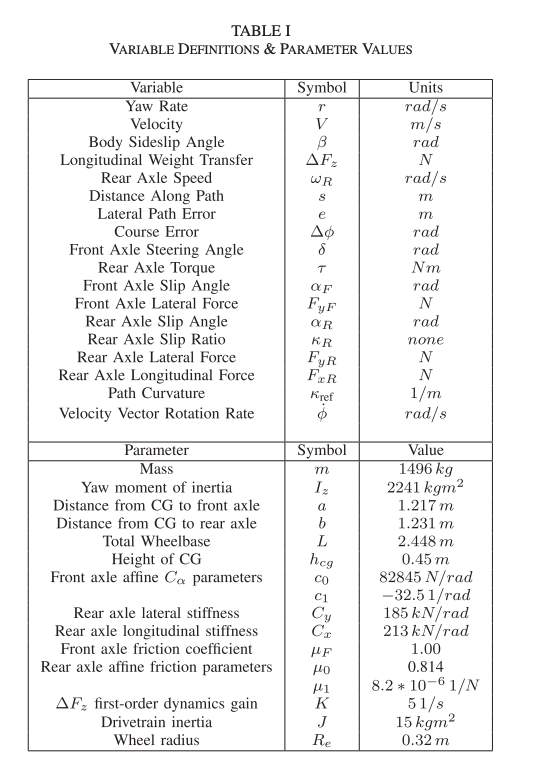
Parameters

• Mass $m$
• Yaw Moment of Inertia $I_z$
• Distance from CG to Front Axle $a$
• Distance from CG to Rear Axle $b$
• Total Wheelbase $L$
• Height of CG
• affine parameters
• etc.

Rear axle force:

• When we talk about forces acting on a turning axle, we’re referring to the interaction between the tires (which are in contact with the ground) and the road surface, NOT forces directly acting on the axle shaft itself

Variables (these capture Vehicle State)

• to write

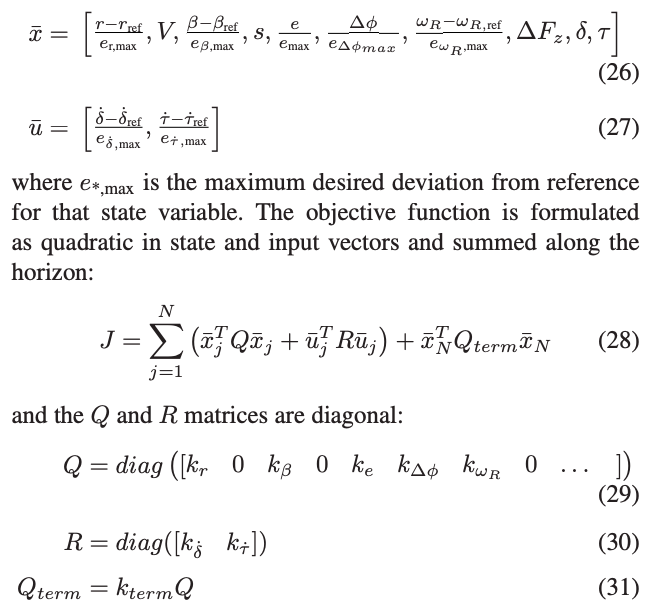
For the optimization, the state vector is $x=[r,V,\beta ,s,e,\Delta \phi ,{\omega }_R,\Delta F_z,\delta ,\tau {]}^T$ and input vector is $u=[\dot{}\delta ,\tau \dot{}{]}^T$.

The state vector and control vectors are slight modified to the following

• Notice that this basically says that velocity is ignored

• $k_r$, $k_{\beta }$, these are hand-tuned gains

Practical tips

• Relatively large costs are put on tracking the desired path (ke) and desired sideslip angle (kβ). A small cost on rear wheelspeed (kωR ) encourages the controller to operate close to the equilibrium wheelspeed and use steering for any small corrections, while kΔφ improves damping in the lateral path tracking state.
• very small cost on yaw rate (kr) aids in convergence time of the nonlinear optimization, while not overly restricting the controller’s ability to use yaw rate to generate sideslip angle.
• Costs on actuator Slew Rate (k_\dot{δ} and k_\dot{τ}) help ensure a smooth closed-loop response.
  • They using the control input as part of the cost that is minimized, to force control inputs to not be super jerky
  • If this was not part of the cost, I think it would be fine, but might be jerky

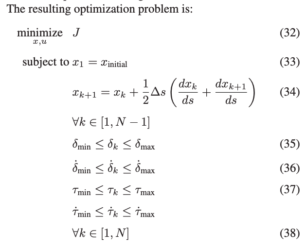
Then the minimization is the following

$k_{term}$​ is a scalar that adjusts the weight of the terminal state cost in the objective function