Linear Classification

Originally, I was like, why am I learning this from CS231N, since I need to work on neural networks. However, I am realizing that the Neural Network are just stacked linear Classifiers (+ Neural Network are just stacked linear Classifiers (+ Activation Function, since they take on the form (called the Neural Network are just stacked linear Classifiers (+ Activation Function, since they take on the form (called the Activation Function, since they take on the form (called the Score Function): $f(x_i,W,b)=W{x}_i+b$

So this will be used as a foundation to understand more complex algorithms. You can think of this as a single classifier that assigns a weight to each pixel with the matrix $W$ and class, i.e. the importance of a particular pixel for a particular class.

Say you want to predict an image of size $(32,32,3)$, (rolled out = $3072$) with $10$ possible classes. You have the following dimensions:

• $x_i$ is $(3072,)$ or more generally $(D,)$
• $W$ are the parameters/weights $(10,3072)$ is or more generally $(C,D)$
• $b$ is the bias term, $(10,)$ or more generally $(C,)$

In practice, we use the Bias Trick to simplify the above expression to $f(x_i,W)=W{x}_i$ by extending the vector $x_i$ with one additional dimension that always holds the constant $1$ - a default bias dimension. With the extra dimension,

• $x_i$ is now $(3073,)$
• $W$ is now $(10,3073)$

Summary of the information flow

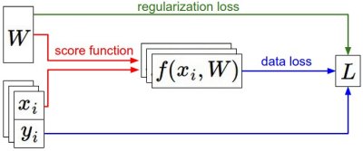
• The dataset of pairs of (x,y) is given and fixed.
• The weights $W$ start out as random numbers and can change.
• During the forward pass the score function computes class scores, stored in vector f.
• The Loss Function contains two components: The data loss computes the compatibility between the scores f and the labels y.
• The regularization loss is only a function of the weights. During Gradient Descent, we compute the gradient on the weights (and optionally on data if we wish) and use them to perform a parameter update during Gradient Descent.
• We want to update $W$ to find a set of weights to minimize the loss function, and then we can use that later to make predictions

Hard Cases for a Linear Classifier

• When you can’t use a line to split a decision boundary, when one class appears in multiple regions of space

Three Views of a Linear Classifier (CS231n)

CS231n insists you can think about $f(x,W)=Wx+b$ in three equivalent ways — each useful for a different intuition.

1. Algebraic view. Just multiply and add. The bias trick (above) collapses $Wx+b$ into a single matmul.

2. Visual view — template matching. Each row of $W$ is itself a $32\times 32\times 3$ image — the template for one class. The score $W_{c,:}\cdot x$ is the inner product of the template with the input image: classification = “which template does my image look most like?” Visualizing rows of $W$ on CIFAR-10 gives you a blurry “average car,” “average horse” (with two heads, since horses face both ways in the data) etc. A linear classifier only gets one template per class — that’s why it’s weak.

3. Geometric view — hyperplanes. Each class score is the signed distance from a hyperplane in pixel space. Decision boundaries are lines (in 2D), planes (3D), hyperplanes (high-D). Two-headed horses → linearly inseparable.

Hard cases (failure modes for a single linear separator)

• Multimodal classes (one class lives in two disconnected regions of pixel space)
• XOR-like configurations
• Concentric rings (class A surrounded by class B)

These motivate everything that follows — multi-template via stacking (MLPs), shift-equivariant templates (CNNs).

Related

• Score Function
• Loss Function
• Softmax Classifier
• Support Vector Machine
• Image Classification
• CS231n

Source

CS231n Lec 2 slides 51–69 (linear classifier, bias trick, three viewpoints, template visualization, hard cases).