A Simple Framework for Contrastive Learning of Visual Representations

How do they prevent mode collapse?

Walkthrough (CS231n 2025 Lec 12)

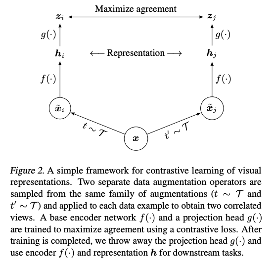
The pipeline

$x\stackrel{t\sim \mathcal{T}}{\to }{\tilde{x}}_i\stackrel{f(\cdot )}{\to }{h}_i\stackrel{g(\cdot )}{\to }{z}_i$

• $\mathcal{T}$ is the augmentation distribution (random crop + color distortion + Gaussian blur — the lec notes these are the crucial three).
• $f(\cdot )$ is the feature encoder (ResNet-50 in the paper). $h$ is what you keep for downstream tasks.
• $g(\cdot )$ is a small MLP projection head. $z$ is where the contrastive loss is applied. Throw $g$ away at inference.

Minibatch algorithm

For a minibatch of $N$ images:

1. Draw $t,t^{\prime }\sim \mathcal{T}$, apply both to every image → $2N$ augmented views.
2. Encode with shared encoder + projection → $z\in {\mathbb{R}}^{2N\times D}$.
3. Build affinity matrix $s_{i,j}=z_i^T{z}_j/(\Vert z_i\Vert \Vert z_j\Vert )$ — cosine similarity, shape $2N\times 2N$.
4. For each row $i$, the positive is at position $2k$ or $2k+1$ (partner view of the same source image); all other $2N-2$ entries are negatives.
5. InfoNCE per row: $\ell (i,j)=-\log \frac{\exp (s_{i,j}/\tau )}{{\sum }_{k\ne i}\exp (s_{i,k}/\tau )}$ Total loss averages $\ell (2k,2k+1)+\ell (2k+1,2k)$ over all $N$ source images.

Why the projection head helps

Representation $z$ is trained to be invariant under augmentation — that collapses useful signal (e.g. color, orientation). $h$ sits one MLP away, so it keeps information that $z$ had to throw out. Linear eval on $h$ beats linear eval on $z$ consistently; SimCLR ablation table shows non-linear projection head ~7 points better than no head.

Why large batch matters

Larger batch = more negatives = tighter MI lower bound ($MI\ge -L-\log N$). Paper sweeps batches from 256 to 8192 and every doubling improves ImageNet linear eval Top-1. Batch 8192 requires TPU pods — the motivation for MoCo’s decoupling trick.

Downstream numbers (Chen 2020)

• Linear eval ImageNet Top-1: SimCLR 69.3% (ResNet-50), SimCLR 4× 76.5% — matches supervised ResNet-50.
• 1% label fine-tune, Top-5: SimCLR 4× 85.8% → beats AlexNet trained with 100× more labels.

Source

CS231n 2025 Lec 12 slides ~76–86, 105–108 (SimCLR architecture + pipeline, minibatch algorithm, affinity matrix, projection head ablation, large-batch ablation, semi-supervised table, summary).

Related

• Contrastive Learning
• Self-Supervised Learning
• MoCo
• Contrastive Loss