State Estimation

Bayes Filter

A Bayes filter is a recursive algorithm that uses Bayes Rule to perform State Estimation.

This was encountered when learning about F1TENTH. Then learned more about this through CS287. Really useful for example to do Localization. Fully understand reading Kalman Filter book.

Kalman Filter Book

Learned about a discrete Bayes filter first, to then understand Kalman Filter afterwards.

We have two fundamental equations for discrete bayes: $\overline{x}=x\ast f_x(\bullet )\text{predict step}$ $x=\Vert L\cdot \overline{x}\Vert \text{update step}$

• $f_x(\bullet )$ is the state propagation function for $x$
• $\ast$ is a Convolution
• $L$ is the likelihood function, $\Vert \Vert$ because we are taking the norm

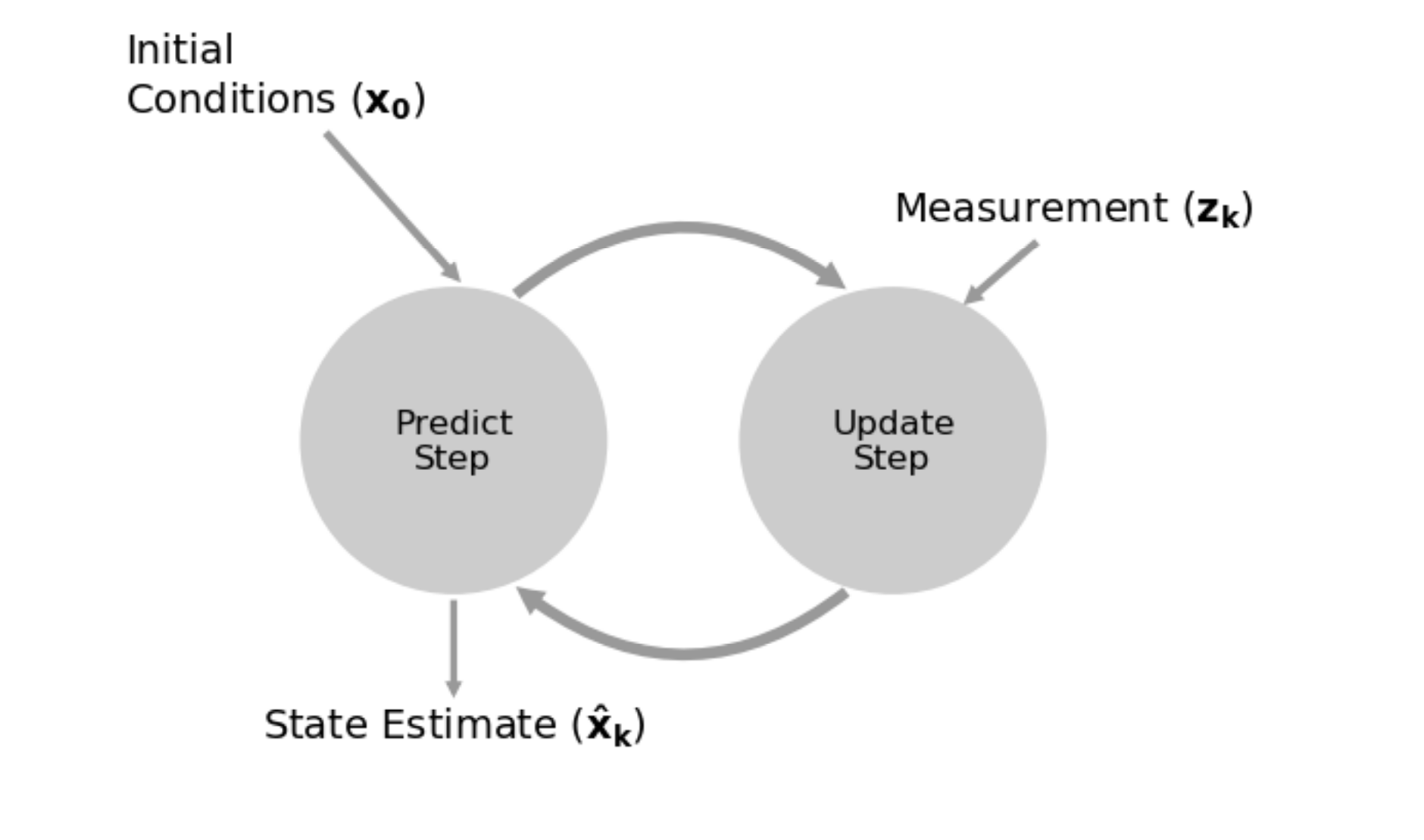
The 2 Major Steps

1. Prediction

• uses the system model to predict the state of the system based on the previous state estimate and the control inputs to the system

2. Update

• uses the current measurement to correct the previous state estimate, and produce a new, more accurate state estimate

Important terminology:

• Prior $\overline{x}$ (prediction)
  • Computed after the predict step
  • Essentially predicting the state purely on your control input, you aren’t measuring anything
• Posterior $x$ (estimated state)
  • Computed from the update step
  • this is refining your estimate based on the new measurements that has come in, which is why it’s called the behavior: new probability given data

Why do we need both predict and update steps?

If we only form estimates from the measurement (update step) then the prediction will not affect the result. If we only form estimates from the prediction (predict step) then the measurement will be ignored.

• If this is to work we need to take some kind of blend of the prediction and measurement.

Here is an example of where you are continually predicting, without making updates. Your belief just ends up converging to no state. This is because you’re not actually using your measurements.

The update step is actually the more crucial component. Predict step is fairly straghtforward.

So how does the update step look like?

def update(likelihood, prior):
    return normalize(likelihood * prior)

How to think of likelihood

Think of likelihood as just your state probability distribution (non-normalized) with your sensor data. Your measurements directly measure state.

posterior = initial_belief()
 
while data_is_available:
    prior = predict(posterior, input)
    likelihood = evaluate_likelihood(measurement, prior)
    posterior = update(likelihood, prior)

• Input is optional and depends on situation, else the predict step is simply setting the prior as 1

Example

For a moving robot, the control input is in the predict step, and the the odometry measurement (wheel enocders) is in the update step

An example for discrete bayes (see chapter 2 for full example)

def discrete_bayes_sim(prior, kernel, measurements, z_prob, hallway):
    posterior = np.array([.1]*10)
    priors, posteriors = [], []
    for i, z in enumerate(measurements):
        prior = predict(posterior, 1, kernel)
        priors.append(prior)
 
        likelihood = lh_hallway(hallway, z, z_prob)
        posterior = update(likelihood, prior)
        posteriors.append(posterior)
    return priors, posteriors

CS287

Given:

• Stream of observations $z$ and action data $u$
• Sensor model $P(z|x)$
• Action model $P(x^{\prime }|u,x)$
• Prior probability of the system state $P(x)$

We want an estimate of the state $X$ of a dynamical system, essentially $P(x|z)$, so we use Bayes Rule

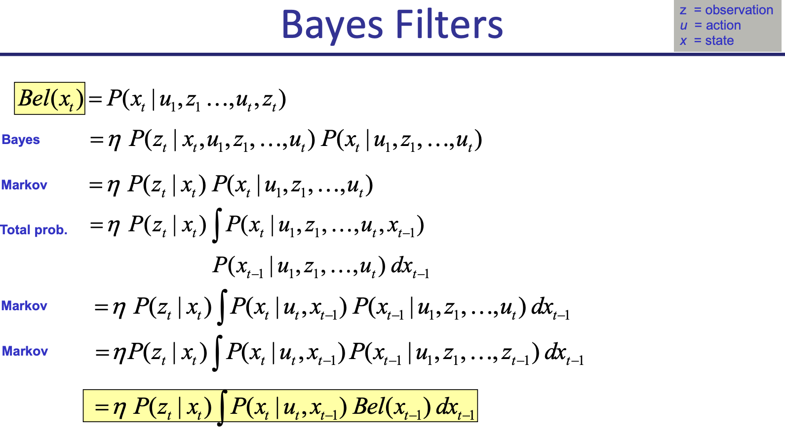
We do doing using by updating the posterior of the state, which we call belief:

$Bel(x_t)=P(x|u_1,z_1,\dots ,u_t,z_t)$

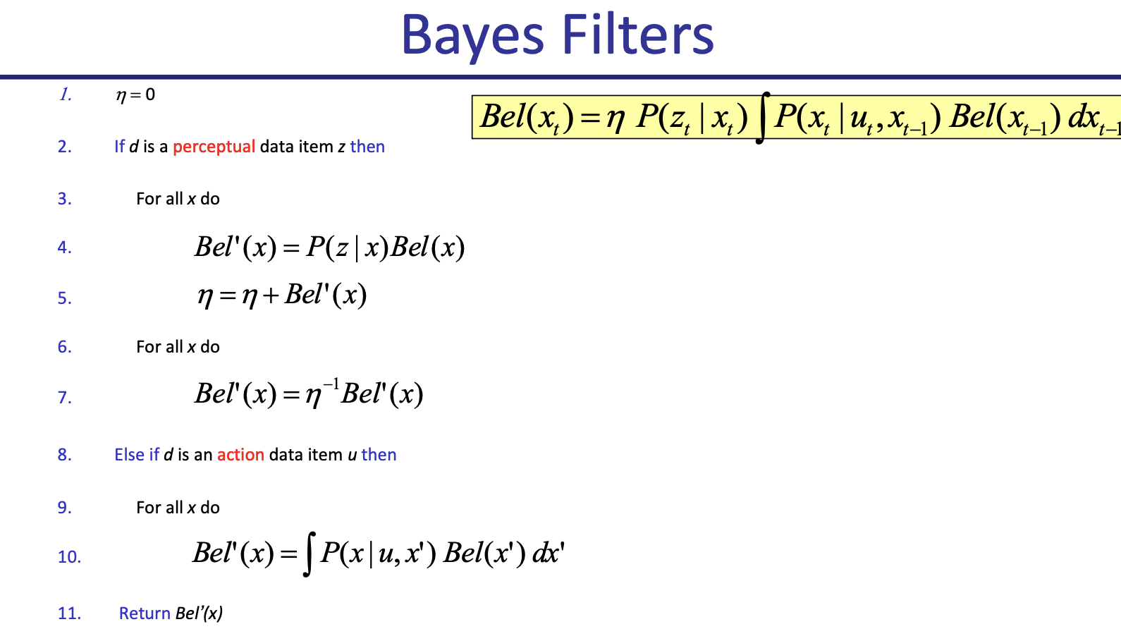
Bayes Filter allow us to recursively update our belief state using the equation $Bel(x_t)=nP(z_t|x_t)\int P(x_t|u_t,x_{t-1})Bel(x_{t-1})d{x}_{t-1}$ where

• $n$ is the normalization constant, to make sure everything adds up to 1
• $p(z_t|x_t)$ is the observation Likelihood sensor model
• Transition model, motion model (simulate noisy dynamics of particles based on control input)

Important

Bayes rule make use of the Markov Assumption.

Derivation from CS287

We can then come up with an algorithm to do this:

Next

• Kalman Filter