State Estimation

Kalman Filter

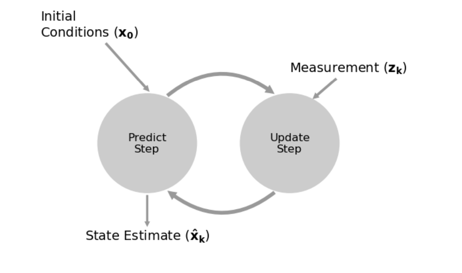
A Kalman filter is a mathematical algorithm for State Estimation based on noisy measurements.

• Recursive algorithm that uses a combination of predictions and measurements to estimate the state of a system over time

Resources

• https://github.com/rlabbe/Kalman-and-Bayesian-Filters-in-Python

Important Idea

“Multiple data points are more accurate than one data point, so throw nothing away no matter how inaccurate it is”

• Ahh so this is also an idea I heard from Steve Macenski

Kalman Filter Book

These 2 chapters most useful:

• Chapter 2: https://github.com/rlabbe/Kalman-and-Bayesian-Filters-in-Python/blob/master/02-Discrete-Bayes.ipynb
• Chapter 4: https://github.com/rlabbe/Kalman-and-Bayesian-Filters-in-Python/blob/master/04-One-Dimensional-Kalman-Filters.ipynb

First understand Discrete Bayes, which helps you build really solid foundation. Everything else builds on top of this. A kalman filter just uses gaussians.

Instead of histograms used with a discrete Bayes filter, we now use gaussians to model the data.

We have two fundamental equations: ${\overline{x}}_N=x_N\oplus f_{x_N}(\bullet )\text{predict step}$ $x=L\otimes {\overline{x}}_N\text{update step}$

• $\oplus$ is gaussian addition, $\otimes$ is gaussian multiplication (see Gaussian Operator)
• $x_N$ indicates that it is gaussian

The basic things

def predict(pos, movement):
    return gaussian(pos.mean + movement.mean, pos.var + movement.var)
    
def gaussian_multiply(g1, g2):
    mean = (g1.var * g2.mean + g2.var * g1.mean) / (g1.var + g2.var)
    variance = (g1.var * g2.var) / (g1.var + g2.var)
    return gaussian(mean, variance)
 
def update(prior, likelihood):
    posterior = gaussian_multiply(likelihood, prior)
    return posterior

# perform Kalman filter
x = gaussian(0., 20.**2)
for z in zs:    
    prior = predict(x, process_model)
    likelihood = gaussian(z, sensor_var)
    x = update(prior, likelihood)
 
    # save results
    predictions.append(prior.mean)
    xs.append(x.mean)

However, this notation is rarely used. Below, we will introduce conversion to conventional Kalman filter notation.

In literature, this is the notation (an alternative but equivalent implementation):

def update(prior, measurement):
    x, P = prior        # mean and variance of prior
    z, R = measurement  # mean and variance of measurement
    
    y = z - x        # residual
    K = P / (P + R)  # Kalman gain
 
    x = x + K*y      # posterior
    P = (1 - K) * P  # posterior variance
    return gaussian(x, P)
 
def predict(posterior, movement):
    x, P = posterior # mean and variance of posterior
    dx, Q = movement # mean and variance of movement
    x = x + dx
    P = P + Q
    return gaussian(x, P)

The kalman gain tells us how much we trust the process vs. the measurement. $K=\frac{P}{P+R}$

https://math.stackexchange.com/questions/1066479/how-to-estimate-variances-for-kalman-filter-from-real-sensor-measurements-withou

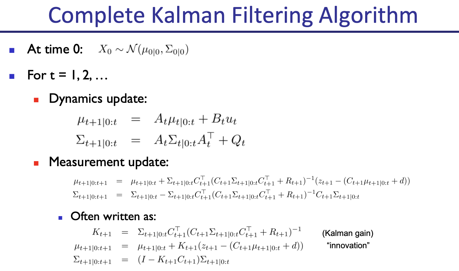
Predict

& \text{(Kalman form)} & \\ \hline \bar \mu = \mu + \mu_{f_x} & \bar x = x + dx & \bar{\mathbf x} = \mathbf{Fx} + \mathbf{Bu}\\ \bar\sigma^2 = \sigma_x^2 + \sigma_{f_x}^2 & \bar P = P + Q & \bar{\mathbf P} = \mathbf{FPF}^\mathsf T + \mathbf Q \\ \hline\end{array}$$ - $\mathbf x,\, \mathbf P$ are the state mean and covariance - correspond to $x$ and $\sigma^2$ - $\mathbf F$ is the state transition function - corresponds to $f_x$ - When multiplied by $\bf x$ it computes the prior - $\mathbf Q$ is the process covariance - corresponds to $\sigma^2_{f_x}$ - $\mathbf B$ and $\mathbf u$ model control inputs to the system > [!note] Addressing discrepancies > > > So I think in the univariate cases, we didn't introduce $Bu$, a possible control input. So then we had $\overline{x} = Fx$ for the multivariate case. Which is fine. But we're also introducing this control input. I was thinking how the control input was $F$, but no, there are like two possible transitions. **Update** $$\begin{array}{|l|l|l|} \hline \text{Univariate} & \text{Univariate} & \text{Multivariate}\\ & \text{(Kalman form)} & \\ \hline & y = z - \bar x & \mathbf y = \mathbf z - \mathbf{H\bar x} \\ & K = \frac{\bar P}{\bar P+R}& \mathbf K = \mathbf{\bar{P}H}^\mathsf T (\mathbf{H\bar{P}H}^\mathsf T + \mathbf R)^{-1} \\ \mu=\frac{\bar\sigma^2\, \mu_z + \sigma_z^2 \, \bar\mu} {\bar\sigma^2 + \sigma_z^2} & x = \bar x + Ky & \mathbf x = \bar{\mathbf x} + \mathbf{Ky} \\ \sigma^2 = \frac{\sigma_1^2\sigma_2^2}{\sigma_1^2+\sigma_2^2} & P = (1-K)\bar P & \mathbf P = (\mathbf I - \mathbf{KH})\mathbf{\bar{P}} \\ \hline \end{array}$$ - $\mathbf H$ is the measurement function - $\mathbf z,\, \mathbf R$ are the measurement mean and noise covariance - Correspond to $z$ and $\sigma_z^2$ in the univariate filter - $\mathbf y$ and $\mathbf K$ are the residual and Kalman gain > [!important] Your job as a designer > > > Your job as a designer will be to design the state $\left(\mathbf x, \mathbf P\right)$, the process $\left(\mathbf F, \mathbf Q\right)$, the measurement $\left(\mathbf z, \mathbf R\right)$, and the measurement function $\mathbf H$. If the system has control inputs, such as a robot, you will also design $\mathbf B$ and $\mathbf u$. ### CS287 I was learning about Kalman Filters back in like Grade 9 when I was trying to build a self-balancing rocket. I watched through quite a few lectures. i was trying to build a [[notes/Rocket Propulsion|Rocket]]. They used those things in rockets! Actually, Kalman filters are used everywhere. Self-driving cars, drones, everything I am interested in actually uses the Kalman filter. From [[notes/CS287|CS287]], a Kalman filter is just a special case of [[notes/Bayes Filter|Bayes Filter]], where dynamics and sensory models linear [[notes/Normal Distribution|Gaussian]]s. ![[attachments/Screen Shot 2022-12-31 at 3.13.18 AM.png]] ### Kalman Filter from Visual SLAM book Notation also used in [[notes/Visual SLAM|Visual SLAM]]. - $u$ is the motion data - $z$ is the observation data - $x$ is the state - $y$ are the landmarks ### Related - [[notes/Extended Kalman Filter|Extended Kalman Filter]]