Autoencoder

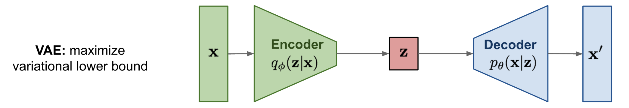
Variational Autoencoder (VAE)

A VAE is a latent variable model trained with variational inference: $p(x)=\int p(x\mid z)p(z)dz$.

Intuition

An autoencoder that forces the latent space to be a well-behaved distribution (usually a unit Gaussian). The KL term pulls the encoder output toward that prior so sampling works; the reconstruction term pushes it to stay informative enough to rebuild the input. The reparameterization trick lets gradients flow through a random sample by pulling the randomness out of the computation graph as a fixed $ϵ$.

What's the reparameterization trick buying us?

Sampling $z$ from a learned distribution is non-differentiable, which breaks backprop. The trick rewrites $z=\mu +\sigma \odot ϵ$ with $ϵ\sim \mathcal{N}(0,I)$, so gradients flow through $\mu ,\sigma$ while randomness lives only in $ϵ$

I got the intuition for VAEs here https://chatgpt.com/share/693a58cf-e2e4-8002-9fea-eb7fad7817b1. A VAE tries to map the original distribution to a Gaussian and back, with both mappings encoded in the loss function.

This is a variant of the Autoencoder that is much more powerful, using distributions to represent features in its bottleneck.

Resources

• https://lilianweng.github.io/posts/2018-08-12-vae/
• https://arxiv.org/pdf/1906.02691

It's basically an Autoencoder but we add Gaussian noise to latent variable z?

Key difference:

• Regular Autoencoder: Input → Encoder → Fixed latent representation → Decoder → Reconstruction
• VAE: Input → Encoder → Latent distribution → Sample from distribution (adds Gaussian noise via reparameterization trick) → Decoder → Reconstruction

Variational autoencoders provide a principled framework for learning deep latent-variable models and corresponding inference models.

Process

Forward Pass (Encoding → Sampling → Decoding)

1. Encoder:
   Input data $x$, outputs parameters (mean and variance) of latent distribution $z$:

$$q_{\varphi }(z|x)=\mathcal{N}(z;{\mu }_{\varphi }(x),{\sigma }_{\varphi }^2(x))$$

2. Reparametrization Trick: Differentiably sample latent variable $z$:

$$z={\mu }_{\varphi }(x)+{\sigma }_{\varphi }(x)\odot ϵ,ϵ\sim \mathcal{N}(0,I)$$

3. Decoder:
   Reconstruct data from sampled latent vector $z$:

$$p_{\theta }(x|z)$$

Loss Function (Negative ELBO):
Optimize encoder and decoder parameters by minimizing:

$$\mathcal{L}(\varphi ,\theta )=-{\mathbb{E}}_{q_{\varphi }(z|x)}[\log p_{\theta }(x|z)]+D_{\text{KL}}(q_{\varphi }(z|x)\Vert p(z))$$

Read the two terms as a tug-of-war. Reconstruction says “encode $x$ into a sharp $z$ so the decoder can recover it”; KL says “but make $q_{\varphi }(z\mid x)$ look like the prior $\mathcal{N}(0,I)$, so I can sample from $p(z)$ at test time and still land on sensible $z$ values.” The balance is what makes the latent space both informative and samplable.

Notes from the guide

The VAE can be viewed as two coupled, but independently parameterized models:

1. encoder (recognition model)
2. decoder (generative model)

Motivation

We want to maximize the log likelihood ${\mathbb{E}}_{x\sim p_{unknwown}}[\log p_{\theta }(x)]$ To make this a generative process, we want it conditioned on some known probability distribution (so then it becomes mapping probability distribution $p(z)$ to $p(x)$) (else it’s just like an Autoencoder, always deterministic).

We expand out $p_{\theta }(x)$: $p_{\theta }(x)=\int p_{\theta }(x,z)dz=\int p_{\theta }(x|z)p_{\theta }(z)dz$

However, this is NOT tractable. Trying every single $z$ value for $p(z)$ is infeasible since $p_{\theta }(x|z)$ is implemented as a neural net.

I'm confused on what is tractable and what is not tractable?

• $p(z)$ is tractable - Simple prior to generate $z$ (i.e. unit gaussian)
• $p(x|z)$ is tractable- simple neural net to general $x$ conditioned on $z$
• $p(x)$ is NOT tractable - need to integrate over all $z$
• $p(z|x)$ is NOT tractable because it needs $p(x)$ applying Bayes Rule

So what do we do? We approximate the intractable posterior $p(z|x)$ with $q_{\varphi }(z|x)$ and maximize a tractable lower bound (ELBO) on the true log-likelihood.

We approximate $q_{\varphi }(z|x)\approx p(z|x)$ and then optimize by maximizing

$p_{\theta }(x)\approx {\mathbb{E}}_{z\sim q_{\varphi }(z|x)}\log p_{\theta }(x|z)$

Variants

• cVAE

Walkthrough (CS231n 2025 Lec 13)

Motivation: from (non-variational) autoencoder to VAE

A plain autoencoder learns features $z$ by training encoder + decoder to reconstruct with L2 loss $\Vert \hat{x}-x{\Vert }_2^2$ (no labels, useful for downstream tasks). But as a generative model it fails:

• If we throw away the encoder and sample $\hat{x}=\text{decoder}(z)$, we need a new $z$. Generating $z$ is no easier than generating $x$, since the encoder has squeezed $x$ into whatever weird-shaped manifold $z$ occupies
• Fix: force $z$ to come from a known distribution (e.g. $\mathcal{N}(0,I)$) so we can sample it trivially

Probabilistic setup

• Prior $p(z)=\mathcal{N}(0,I)$: simple, samplable
• Decoder $p_{\theta }(x\mid z)=\mathcal{N}({\mu }_{x|z},{\sigma }^{2}I)$: a neural net outputting a mean, so $\log p_{\theta }(x\mid z)=-\frac{1}{2{\sigma }^2}\Vert x-\mu {\Vert }^2+C$, meaning maximizing log-likelihood under a Gaussian decoder equals minimizing L2 reconstruction
• Encoder $q_{\varphi }(z\mid x)=\mathcal{N}({\mu }_{z|x},{\Sigma }_{z|x})$: a neural net outputting mean + (diagonal) variance of the approximate posterior

Marginal $p_{\theta }(x)=\int p_{\theta }(x\mid z)p(z)dz$ is intractable (can’t integrate over all $z$). Bayes’ rule $p_{\theta }(x)=p_{\theta }(x\mid z)p(z)/p_{\theta }(z\mid x)$ has $p_{\theta }(z\mid x)$ which is also intractable. So we introduce $q_{\varphi }(z\mid x)\approx p_{\theta }(z\mid x)$ and maximize the ELBO instead.

Training objective

$\boxed{\mathcal{L}=\underset{\text{reconstruction}}{\underbrace{{\mathbb{E}}_{z\sim q_{\varphi }(z|x)}[\log p_{\theta }(x\mid z)]}}-\underset{\text{prior matching}}{\underbrace{D_{\text{KL}}(q_{\varphi }(z\mid x)\Vert p(z))}}}$

Both terms are closed-form for Gaussians (the KL between two diagonal Gaussians has a known formula), except the expectation over $z$, which we Monte-Carlo with the reparametrization trick $z={\mu }_{z|x}+ϵ\odot {\Sigma }_{z|x}^{1/2}$, $ϵ\sim \mathcal{N}(0,I)$.

Training loop

1. $x\to$ encoder $\to {\mu }_{z|x},{\Sigma }_{z|x}$
2. Prior loss: KL-pull $q_{\varphi }(z\mid x)$ toward $\mathcal{N}(0,I)$
3. Sample $z$ via reparametrization (so gradients flow through $\mu ,\Sigma$)
4. $z\to$ decoder $\to {\mu }_{x|z}$
5. Reconstruction loss: L2 between ${\mu }_{x|z}$ and $x$

The two losses fight each other

• Reconstruction wants ${\Sigma }_{z|x}\to 0$ and a unique ${\mu }_{z|x}$ for each $x$ (so the decoder can reconstruct deterministically, essentially a plain autoencoder)
• Prior matching wants ${\Sigma }_{z|x}=I$ and ${\mu }_{z|x}=0$ for every $x$ (so $q_{\varphi }(z\mid x)=p(z)$ and sampling is easy)

The balance between them is what makes VAEs generative rather than just compressive.

Sampling

At inference, throw away the encoder. Sample $z\sim \mathcal{N}(0,I)$, run through the decoder, get a new image.

Disentangling

Because the prior $p(z)=\mathcal{N}(0,I)$ has a diagonal covariance, the dimensions of $z$ are forced to be independent. Walking one dimension at a time often maps to a human-interpretable factor (digit identity, stroke width, pose). Kingma & Welling’s ICLR 2014 MNIST grid, varying $z_1$ vs $z_2$ to smoothly trace through digit classes and styles, is the canonical demo.

From CS231n 2025 Lec 13 slides ~62-112 (non-variational AE recap, motivation for forcing known prior, encoder/decoder Gaussian parameterization, log-likelihood $\to$ L2 equivalence, ELBO derivation via Bayes + multiply-by-$q$, training steps with KL prior / reparametrization / reconstruction, “losses fight” interpretation, sampling procedure, disentangling MNIST grid).

Related

• ELBO
• Reparametrization Trick
• Autoencoder
• Generative Model
• KL Divergence