Flow-Based Model

Normalizing Flow

A normalizing flow transforms a simple distribution (generally a Unit Gaussian) into a complex, data-like distribution using a sequence of invertible and differentiable functions.

Intuition

Build a complex distribution by stacking invertible transforms on a simple one (Gaussian). Because every transform is invertible and you can compute its Jacobian, you get exact log-likelihoods via change of variables, unlike GANs (no density) or VAEs (only a lower bound). The price: every layer has to be invertible, which constrains the architecture (coupling layers, 1×1 convs, etc.)

Why an invertible transform instead of a separate encoder/decoder?

Invertibility lets us evaluate exact log-likelihood via change of variables, so training is MLE with a tractable objective, no ELBO or adversary needed

This is an idea I saw Billy Zheng write about: https://hongruizheng.com/2020/03/13/normalizing-flow.html

Resources

• https://lilianweng.github.io/posts/2018-10-13-flow-models/

Normalizing flow learns an invertible transformation $f$ between data and latent variables: $x=f(z),z=f^{-1}(x)$

where:

• $x$ is a data sample
• $z$ is a latent variable sampled from a simple distribution

You can't just have z

The function $f$ in normalizing flows is perfectly invertible. We care about density estimation, not reconstruction. The loss is based on the log-likelihood of data $x$ under the model (more below). A flow with a separate encoder/decoder would basically be an Autoencoder

We can write this in terms of probability density function (comes from the Change-of-Variable Formula theorem in probability): $x=f(z),p(x)=p(z)\left|\det \left(\frac{\partial f^{-1}}{\partial x}\right)\right|$

Geometric picture

Probability mass has to be conserved. If $f$ stretches a tiny volume around $z$ by a factor of $|\det J|$, the density at $f(z)$ must drop by the same factor so the total still integrates to 1. The Jacobian determinant is exactly the local volume-stretch of the transform.

Where does \det(\frac{\delta f^{-1}}{\delta x}) come from?

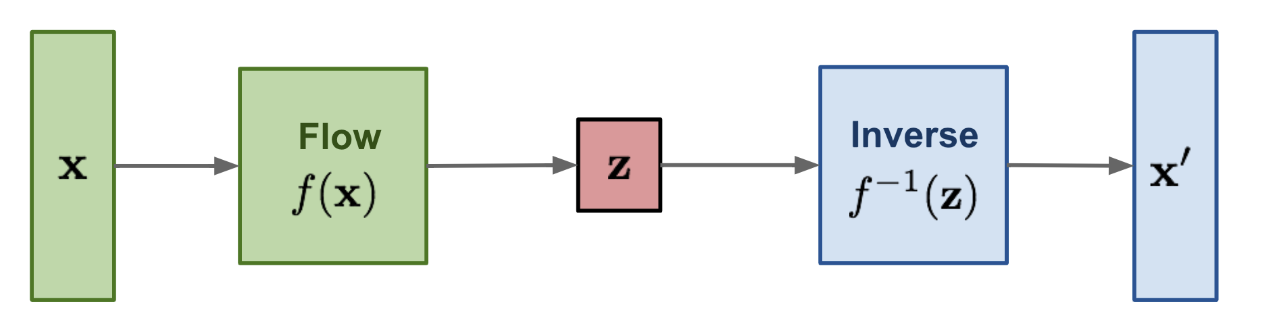
• In training, data flows $x\to z$: apply the inverse flow $z=f^{-1}(x)$ and minimize the loss over $f^{-1}$. Compute the Log Likelihood using the change-of-variable formula: $\log p_X(x)=\log p_Z(z)+\log \left|\det \left(\frac{\partial f^{-1}}{\partial x}\right)\right|$. Notice the magic, because below, we can then use $f$, all thanks to the fact that $f$ is invertible
• In sampling / generation, data flows $z\to x$: sample $z\sim \mathcal{N}(0,I)$ from the base distribution and apply the forward flow $x=f(z)$

Difference with VAE?

It comes down to how we formulate the loss. In a VAE the encoder and decoder are separate networks:

• Normalizing flow is deterministic: no randomness is added when transforming $x\leftrightarrow z$, we know exactly what happens
• VAE is stochastic: the encoder samples $z$ from a learned distribution $q(z|x)$ and outputs a distribution

Both model Gaussians:

• In flows, the Gaussian is transformed through exact, invertible functions to match the data
• In VAEs, the model approximates the mapping between data and latent Gaussian through separate encoder/decoder networks

Sampling:

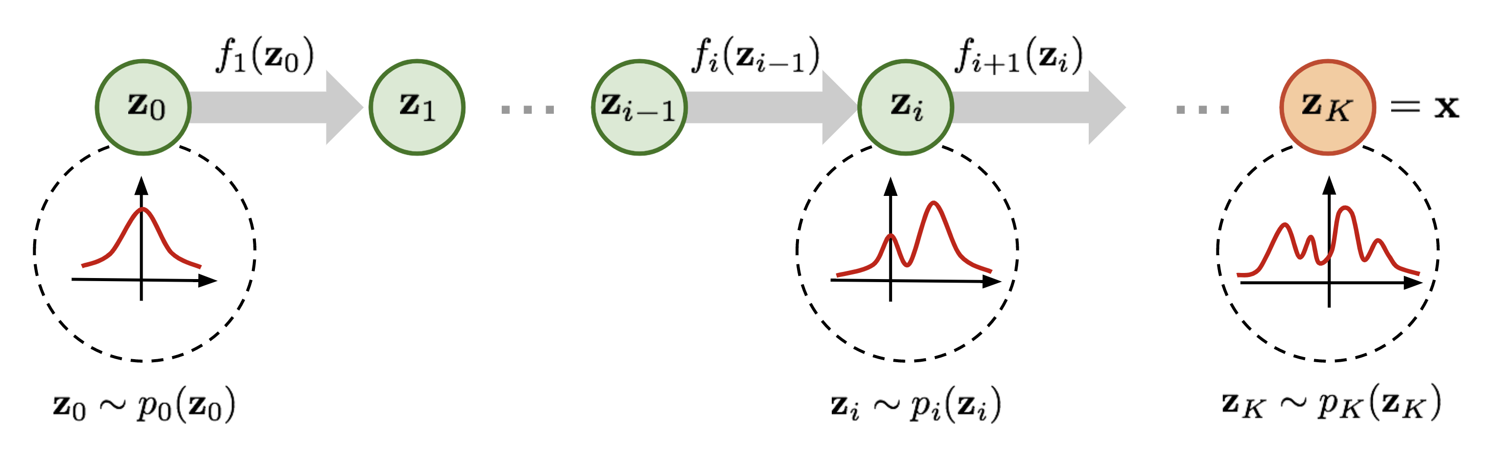We apply a chain of invertible transformations:

$$\mathbf{x}=f_K\circ f_{K-1}\circ \cdots \circ f_1({\mathbf{z}}_0)$$

where:

• ${\mathbf{z}}_0\sim \mathcal{N}(0,I)$ is a latent variable sampled from a standard Gaussian
• Each $f_i$ is an invertible transformation (e.g. affine coupling layer)
• Output $\mathbf{x}$ is a realistic-looking data sample

What does $f$ look like? Depends on the model. They’re generally just Affine Transforms, since those are differentiable.

The trick of a coupling layer: split the input in half, leave the first half alone, and use it to compute a scale $s$ and shift $t$ for the second half. The first half is unchanged, so inversion is trivial; and because only ${\mathbf{x}}_b$ depends on ${\mathbf{x}}_a$ (not vice versa), the Jacobian is triangular and its determinant is just the product of the diagonal ($\exp (s_{\theta })$ entries). That’s why $s_{\theta },t_{\theta }$ can be arbitrarily complex neural nets without wrecking invertibility.

Forward pass:

$$\begin{array}{rl}{\mathbf{y}}_a& ={\mathbf{x}}_a\\ {\mathbf{y}}_b& ={\mathbf{x}}_b\odot \exp (s_{\theta }({\mathbf{x}}_a))+t_{\theta }({\mathbf{x}}_a)\end{array}$$

Inverse pass:

$$\begin{array}{rl}{\mathbf{x}}_a& ={\mathbf{y}}_a\\ {\mathbf{x}}_b& =({\mathbf{y}}_b-t_{\theta }({\mathbf{y}}_a))\odot \exp (-s_{\theta }({\mathbf{y}}_a))\end{array}$$

where:

• $s_{\theta }$ and $t_{\theta }$ are neural networks (often small CNNs or MLPs)
• Same parameters are reused in both directions

How Weight Updates Work in Flow-Based Models

Training is done via maximum likelihood estimation (MLE) using the change-of-variables formula.

Change of Variables

Given $\mathbf{x}=f(\mathbf{z})$ and $\mathbf{z}\sim \mathcal{N}(0,I)$:

$$\log p_X(\mathbf{x})=\log p_Z(f^{-1}(\mathbf{x}))+\log \left|\det \left(\frac{\partial f^{-1}}{\partial \mathbf{x}}\right)\right|$$

Rewriting using forward Jacobian:

$$\log p_X(\mathbf{x})=\log p_Z(\mathbf{z})-\log \left|\det \left(\frac{\partial f}{\partial \mathbf{z}}\right)\right|$$

The fundamental difference

This loss uses a Jacobian, derived from the change of variables formula. We’re not just doing $L=x-f(z)$

Training Steps

1. Inverse pass: given data $\mathbf{x}$, compute $\mathbf{z}=f^{-1}(\mathbf{x})$
2. Compute log-likelihood loss:

$$\mathcal{L}=-\log p_Z(\mathbf{z})+\log \left|\det \left(\frac{\partial f}{\partial \mathbf{z}}\right)\right|$$

3. Backpropagate through:
   • the inverse transformations $f^{-1}$
   • the neural nets $s_{\theta }$ and $t_{\theta }$
   • the log-determinant term (structured for easy computation in RealNVP/Glow)
4. Gradient Descent: use Adam/SGD to update parameters $\theta$ in $s_{\theta }$ and $t_{\theta }$

Normalizing flow gives you an explicit representation of density functions.

• Kernel Density Estimation

Used a lot in Generative Model.

Related

• Flow Matching