NumPy

Super useful in the Data Science world. Used at Data Science world. Used at Ericsson.

I get so confused on indexing, see Indexing on Arrays

https://www.pythonlikeyoumeanit.com/Module3_IntroducingNumpy/VectorizedOperations.html

Two courses where I really needed to get good at this, this is why Linear Algebra is super important

• CS231N
• CS287

Things I don’t know:

• np.squeeze ? → Remove axes of length one
  • opposite is expand_dims
• np.meshgrid → introduced in CS287

Operations I need to master and use on a day-to-day:

• Master understanding of broadcasting
• np.where
• Advanced indexing using X[np.arange(N), y]
• np.random.choice
• np.mean(y_train_pred == y_train)
• np.linspace → never used it myself, but I see it being used
• np.randn()
• np.reshape() (more details below)
  • If you want to reshape to another numpy array dimension, just pass that array’s shape as the argument!

Transpose vs reshaping?

Broadcasting trick: use keepdims=True instead of having to use the transpose in case of shape mismatch.

For example, with the Softmax Function, assume x is a matrix of $N$ samples of dimension $D$, i.e. $(N,D)$, we want to return a softmax vector for each sample:

def stable_softmax(x): # Assumes x is a vector
    z = X - max(x, axis=1, keepdims=True) # This is much better than z = (X.T - max(X,axis=1)).T
    exps = np.exp(z)
    return exps/np.sum(exps)

NumPy’s ND-arrays are homogeneous, i.e.  they only contain data of a single type. Thanks to this restriction on types, NumPy can optimize the mathematical operations in compiled C code. This is a process that is referred to as Vectorization.

Python painstakingly checks the data type of every one of the items as it iterates over the arrays since it typically works with lists with unrestricted contents.

Note

However, NumPy code only runs on CPU. This is why frameworks like Tensorflow and Pytorch exist to have the code run on GPU, to do more parallel operations.

Set the seed, so every time, the random number created is the same.

np.random.seed(0)

Always use vectorized functions when possible

We should avoid performing explicit for-loops over long sequences of data in Python, be them lists or NumPy arrays, when we can use vectorized functions.

What this does is that when Python compiles to C-code, it parallelizes some of the operations.

Axis

It was hard for me to visualize the axis, when you do like Numpy.sum. However, I have this picture in my head:

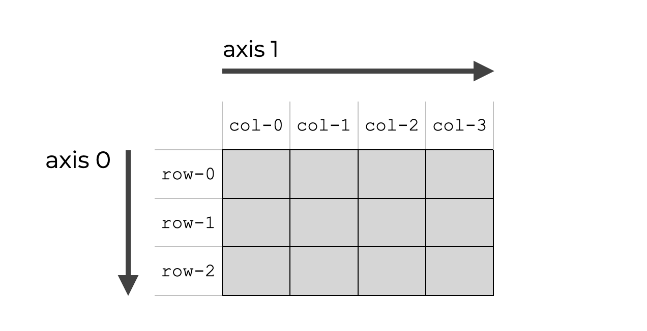
So when specify a particular axis, you sum along a particular dimension, when the axis represent the n-th dimension. By default, np.sum sums alongside every single axis.

If it is a 3D shape, you have up to 3-axes (0,1,2) to choose from.

Indexing on Arrays

This is the most important. I keep getting confused. https://numpy.org/doc/stable/user/basics.indexing.html

For a 2D array, x[0, 2] == x[0][2]. However, the second case is more inefficient as a new temporary array is created after the first index that is subsequently indexed by 2.

However, x[:, i] vs x[:][0] are NOT the same, they do not produce the same outputs. Consider the following example `

import numpy as np
a = np.array([[1,2], [3,4]])
"""
[[1,2]
 [3,4]]
"""
 
a[:, 0] # [1,3] gets the first column
a[:][0] # [1,2], gets the first row
a[0, :] # [1,2] gets the first row

But I don’t get the difference with the np.arange vs :. I’ve done exercises through cs231n and get a better understand, but look at advanced indexing on numpy page to get better understanding. Also see right below

Okay, now I get it:

• If you use like x[:, 5], this means that select all rows, and the 5th column for all values
• If you use like x[np.arange(4), [0,1,2,3]] → this is like you select specific values using the (row, column) pairs that will be generated. So make sure that are both the same shape

Consider the follow example:

a = np.array([[1,2],[3,4]])
"""
array([[1,2],
	  [3,4]])
"""
 
a[np.arange(2), [0,0]] # [1,3] intended behavior. -> See this https://numpy.org/devdocs/user/basics.indexing.html#slicing-and-striding. np.arange(2) returns an array [0,1], so you use the first as indices for the rows, and the second as indices for the columns.
"""
a[np.arange(2), [0,0,0]] would return an error
"""
 
 
a[:, [0,0]] # [[1,1], [3,3]] NOT intended behavior -> take all the rows, and then storing each row in a new matrix where each row has the values [0th-index, 0th-index]
 
# You can do 
a[:, 0] # this would return [1,3] the intended behavior
 

I think the reason I am confused is I would do this in Pandas, and that also works in NumPy. However, with more complex vectorization problems, you need advanced indexing, which is what you see above.

X = dataset.iloc[:, 3:13].values
y = dataset.iloc[:, 13].values

More examples, for a 3D matrix, updating multiple values at the same time, by just indexing

a = np.zeros((20,25,40))
a[0,0, [1,3,4]] = [60, 40, 20]
a[0,0, [1,3,4]] = [20, 30] # ERROR, you are trying to update 3 different values with 2 values

Using another array to index

a = np.array([[1, 2],
           [3, 4]])
b = np.array([1,1])
 
a[tuple(b)]

Broadcasting

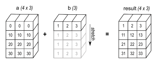
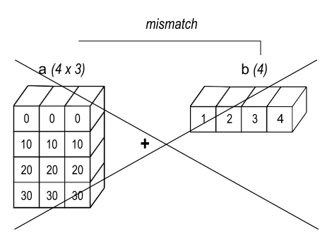
When operating on two arrays, NumPy compares their shapes element-wise. It starts with the trailing (i.e. rightmost) dimensions and works its way left. Two dimensions are compatible when

1. they are equal, or
2. one of them is 1

“Align all the dimensions, starting from the right”. https://numpy.org/doc/stable/user/basics.broadcasting.html

NumPy provides a mechanism for performing mathematical operations on arrays of unequal shapes. An array will be treated as if its contents have been replicated along the appropriate dimensions, such that the shape of this new, higher-dimensional array suits the mathematical operation being performed.

We don’t need to redundantly copy the contents, which makes broadcasting fast.

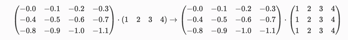
Ex: (3,4) times (4) → (3,4) matrix

Some more examples:

• shape-(3, 1, 2) multiplied with shape-(3, 1) → (3,3,2)
• shape-(8) multiplied with shape-(5,2,8) → (5,2,8)
• shape-(8,1,3) multiplied with shape-(8,5,3) → (8,5,3)

Broadcasting two arrays together follows these rules:

1. If the arrays do not have the same rank, prepend the shape of the lower rank array with 1s until both shapes have the same length.
2. The two arrays are said to be compatible in a dimension if they have the same size in the dimension, or if one of the arrays has size 1 in that dimension.
3. The arrays can be broadcast together if they are compatible in all dimensions.
4. After broadcasting, each array behaves as if it had shape equal to the elementwise maximum of shapes of the two input arrays.
5. In any dimension where one array had size 1 and the other array had size greater than 1, the first array behaves as if it were copied along that dimension

Reshaping

I actually need to understand how reshaping is actually done, because I did reshaping and there are actually three ways to reshape.

order = ‘C’

• The C actually stands for the programming language C. This is the default order and if we type:

order = ‘F’

• The F actually stands for the programming language Fortran.
• In the Fortran order, we unroll by changing the first index fastest, the second index the last index changing slowest

print(a.reshape([4, 6], order='C'))
# [[ 0  1  2  3  4  5]
#  [ 6  7  8  9 10 11]
#  [12 13 14 15 16 17]
#  [18 19 20 21 22 23]]
 
print(a.reshape([4, 6], order='F'))
# [[ 0  4  8 12 16 20]
#  [ 1  5  9 13 17 21]
#  [ 2  6 10 14 18 22]
#  [ 3  7 11 15 19 23]]

order = ‘A’

• idk, it’s like a combination of both