Counterfactual Regret Minimization

https://nn.labml.ai/cfr/index.html

CFR is an extension of Regret Matching for extensive-form games. We use CFR to solve Imperfect Information games, i.e. cases where the game is only partially observable, such as Poker.

This is a really good paper to introduce your to CFR, and a tutorial here.

Link to original paper:

• http://poker.cs.ualberta.ca/publications/NIPS07-cfr.pdf
• https://papers.nips.cc/paper/2007/file/08d98638c6fcd194a4b1e6992063e944-Paper.pdf

This is good blog:

• https://int8.io/counterfactual-regret-minimization-for-poker-ai/
• You should look at MCCFR http://mlanctot.info/files/papers/nips09mccfr.pdf
  • They explain CFR in there. I think you should understand the theory behind the regret bounds, even if it is going to take a bit of time. Because I don’t want to be a scam. I want to truly understand what I am doing

Families of CFR

• Monte-Carlo CFR
• CFR-D (CFR-decomposition) (2014)
  • allows “sub-linear space costs at the cost of increased computation time”
• CFR+ (2015) used to solve Heads Up Limit Hold’Em
  • all regrets are constrained to be non-negative
  • Final strategy used is the current strategy at that time (not the average strategy)
  • no sampling is used
• Discounted CFR(2018)
• Instant CFR (2019)
• Deep CFR (2020?)

Connection between Regret, average strategies, and Nash Equilibrium

In a zero-sum game, if $R_{i\in \{1,2\}}^T\le ϵ$, then ${\overline{\sigma }}^T$ is a $2ϵ$ equilibrium.

Two papers have been used to produce the article below:

• Regret Minimization in Games with Incomplete Information: The original paper that came up with the counterfactual regret minimization algorithm.
• Monte Carlo Sampling for Regret Minimization in Extensive Games: introduces Monte Carlo Counterfactual Regret Minimization (MCCFR), where we sample from the game tree and estimate the regrets.

The notation written below is entirely taken from the papers above. If you want the original source of truth to produce this article, refer to the original papers. The goal of this article is to produce a more user-friendly introduction, as well as for my own self-learning.

Credits to LabML’s annotated CFR for the original idea to host a this style of notebook. Contents are very similar.

See Poker AI Blog, where we first talk about RPS and regret matching. I think it is helpful to go through that first, but not necessary.

#todo Check-out Lilian Weng’s blog, and Andrej Karpathy’s blog, and see how much notation they use.

Extensive-Form Game with Imperfect Information

Before we dive into the CFR algorithm, we need to first formally the game we are trying to solve. A basic understanding of notation behind Functions, Relations and Sets is needed to grasp the notation below (if rusty, check out a quick cheatsheet here).

No-Limit Texas Hold’Em Poker is a finite extensive game with imperfect information:

• Finite because we can guarantee that the game will terminate
• Extensive because there are multiple decisions made in a single game, unlike Rock Paper Scissors, which is called a normal-form game
• Imperfect Information because each player can only make partial observations, i.e they cannot see the other player’s cards

A finite extensive game with imperfect information has the following components):

1. A finite set $N$ of Players
2. A finite set $H$ of Histories
3. A Player Function
4. A Chance Function
5. Information Sets
6. Utility Function

Player

An imperfect information extensive game (IIEG) has a finite set $N$ of players.

• We denote a particular player by $i$, where $i\in N$
• For Heads-Up Poker, there are only two players, so $N=\{0,1\}$

History

An IIEG has finite set $H$ of possible histories of actions.

• Each history $h\in H$ denotes a sequence of legal actions
• $Z$ is the set of terminal histories, $Z\subseteq H$, i.e. when we have reached the end of a game
• $A(h)=\{a:(h,a)\in H\}$ is the set of actions available after a non-terminal history $h\in H$#todo you have both $h$ and $(h,a)$ which is confusing

Player Function

A player function $P:H\setminus Z\to N\cup \{c\}$ assigns each nonterminal history $h\in H\setminus Z$ to an element of $N\cup \{c\}$, which tells you whose turn it is

• When $P(h)\in Z$, the function returns the player who has to take an action after non-terminal history $h$
• When $P(h)=c$, then chance determines the action taken after history $h$
  • This is when for example, it is time to draw a new card. It is not up to the player to decide

Chance Function

• A function $f_c:H\to \mathbb{R}$ that assigns a probability measure $f_c(a|h)$ for all $a\in A(h)$, for each history $h$ where $P(h)=c$. In Poker, this simply assigns an equal probability for each card of the remaining deck that gets drawn.

Information Set

• An information partition ${\mathcal{I}}_i$ of $\{h\in H:P(h)=i\}$ for each player $i\in N$, where $A(h)=$A(h’)$whenever$h$and$h’$ are members of the same partition
  • #gap-in-knowledge information partition is confusing, what is this??
  • Each information set $I_i\in {\mathcal{I}}_i$ for player $i$ contains a set of histories that look identical to player $i$
    • Note that we will often just write $I$ instead of $I_i$

Utility

A utility function $u_i:Z\to \mathbb{R}$ for each player $i\in N$

• The function $u_i(z)$ returns how much player $i$ wins/loses at the end of a game given a terminal history $z\in Z$
• ${\Delta }_{u,i}={\max }_z(z)-{\min }_z{u}_i(z)$ is the range of utilities to player $i$
• when $u_1=-u_2$, and $N=\{1,2\}$, we have a zero-sum extensive game (such as in the case of Heads-Up Poker)

Some Clarifications:

• when you are initially dealt two cards, that is part of the history. Then, your opponent gets dealt two cards. However, you won’t be able to see that information about the history.

Strategy and Equilibria

Now that we have formally defined the notation for the extensive game, let us define strategies to play this game:

Strategy

• A strategy ${\sigma }_i$ of player $i$ is a function that assigns a distribution over $A(I)$ for each $I\in {\mathcal{I}}_i$
  • As player $i$, we follow our strategy ${\sigma }_i$ to decide which action to pick throughout the game
  • ${\sigma }_i(I,a)$ represents the probability of choosing action $a\in A(I)$ given information set $I$ for player $i$
  • Two types of strategies:
    • Pure strategy (deterministic): Chooses a single action with probability 1.
    • Mixed strategy ($\sigma$): At least two actions played with positive probability
• ${\sum }_i$ is the set of all strategies for player $i$

Parallel: If you’ve dabbled/are an expert in reinforcement learning, strategy corresponds to the policy $\pi$ that an agent follows, where $\pi (a|s)$ represents the probability of choosing action $a$ given that the agent is in state $s$.

However, in Game Theory, we use $\pi$ to denote reach probability (see more below).

Strategy Profile

• A strategy profile $\sigma$ consists of a strategy for each player ${\sigma }_1,\dots ,{\sigma }_n$
• ${\sigma }_{-i}$ refers to all the strategies in strategy profile $\sigma$ excluding ${\sigma }_i$

Reach Probability of History

This is a really crucial idea that one must understand before moving on.

• ${\pi }^{\sigma }(h)$ is the reach probability of history $h$ (probability of $h$ occurring) if all players choose to play according to strategy $\sigma$ ${\pi }^{\sigma }(h)={\Pi }_{i\in N\cup \{c\}}{\pi }_i^{\sigma }(h)$ In other words, it’s the probability of each player multiplied together. But shouldn’t it be the contribution from both players? So draw out Rock papers scissors and the probabilities. Example: ${\sigma }_1=[\frac{1}{3},\frac{1}{3},\frac{1}{3}]$, ${\sigma }_2=[\frac{1}{3},\frac{1}{3},\frac{1}{3}]$, where the actions are $[Rock,Paper,Scissors]$ If each player plays RPS with 1/3 probability, then $\pi ([R])=1/3$ Player 2 doesn’t play at this point, so how do you compute ${\pi }_2^{\sigma }(h)$?
• Well, the probability is just 1

so its actually Let’s decompose $h=h_1{h}_2{h}_3\dots h_n$ ${\pi }^{\sigma }(h)={\pi }_1^{\sigma }(h_1){\pi }_2^{\sigma }(h_1{h}_2){\pi }_1^{\sigma }(h_1{h}_2{h}_3)\dots$

So say it’s Rock Rock. From the perspective We actually only know $\sigma (I,a)$ like what

This is telling the probability that you are to end up in history $h$.

The probability of reach an information set $I$ under strategy profile $\sigma$ given by ${\pi }^{\sigma }(I)={\sum }_{h\in I}{\pi }^{\sigma }(h)$

• Notice that the above is a sum, and not a product, because multiple histories can be the same InfoSet, so we increase our chances of encountering a particular information set by summing the probabilities.

We also define ${\pi }^{\sigma }(h,z)$, the reach probability of a terminal history $z$ given the current history $h$ under strategy profile $\sigma$: ${\pi }^{\sigma }(h,z)=\{\begin{array}{ll}\frac{{\pi }^{\sigma }(z)}{{\pi }^{\sigma }(h)}& h⊑z\\ 0& \text{otherwise}\end{array}$

Expected Payoff

The utility function we covered gives us some payoff $u_i(z)$ for player $i$ at terminal history $z\in Z$. How can we measure our average payoff as we play the game more and more? That is the idea of an expected payoff.

The expected payoff for player $i$ is given by $u_i(\sigma )={\sum }_{h\in Z}{u}_i(h){\pi }^{\sigma }(h)$

This is simply a single value that tells you how good your strategy profile $\sigma$. That is, if you play according to $\sigma$, how much money do you expect to win or lose? our goal is to reach a Nash Equilibrium, so $u_i(\sigma )=0$.

• Intuitively, we are simply taking a weighted average, multiplying our payoff $u_i(h)$ of each terminal history $h\in Z$ by how likely we are to reach that history using strategy profile $\sigma$, given by ${\pi }^{\sigma }(h)$. Note that ${\sum }_{h\in Z}{\pi }^{\sigma }(h)=1$.
• The expected payoff is different depending on what strategy profile $\sigma$

We will also sometimes use the notation $u_i({\sigma }_i,{\sigma }_{-i})$, which is the expected payoff for player $i$ if all players play according to the strategy profile $\sigma =⟨{\sigma }_i,{\sigma }_{-i}⟩$.

• We use this expanded form because we will also add a superscript $t$ in \sigma^\textcolor{orange}{t}_i, so you can obtain the utility at two different times, for example $u_i({\sigma }_i^{t-1},{\sigma }_{-i}^t)$

We can also talk about expected payoff $u_i(\sigma ,h)$ at a particular nonterminal history $h$ (this is also sometimes referred to as just expected value at a particular history $h$) $v_i(\sigma ,h)=u_i(\sigma ,h)={\sum }_{z\in Z,h⊏z}{\pi }_{-i}^{\sigma }(h){\pi }_i^{\sigma }(h,z)u_i(z)$ We also call the above counterfactual value at nonterminal history $h$, but instead of histories, we are interested in getting the value for an information set $I$.

$v_i(\sigma ,I)={\sum }_{z\in Z_I}{\pi }_{-i}^{\sigma }(z[I]){\pi }^{\sigma }(z[I],z)u_i(z)$

• I am quite confused by why this equation is the way it is, so you should see below for counterfactual value.

Serendipity: This is quite similar to the value functions we see in Reinforcement Learning, where we do a Monte-Carlo rollout to sample the rewards.

Some more notes about discrepancies

Note: Notice that we were defining the domain of utility function $u_i$ as the set of terminal histories $Z$, but now we define it as a strategy profile.#todo Explain discrepancy.

Nash Equilibrium

Our goal is to find the Nash Equilibrium. This is a strategy profile in which no players can improve by deviating from their strategies.

Formally, in a two-player extensive game, a Nash Equilibrium is a strategy profile $\sigma$ where the two inequalities are satisfied: $\{\begin{array}{l}{u}_1(\sigma )\ge {\max }_{{\sigma }_1^{\prime }\in {\sum }_1}{u}_1({\sigma }_1^{\prime },{\sigma }_2)\\ u_2(\sigma )\ge {\max }_{{\sigma }_2^{\prime }\in {\sum }_2}{u}_2({\sigma }_1,{\sigma }_2^{\prime })\end{array}$

• For instance, the first equation states for take any strategy ${\sigma }_1^{\prime }$ for player $1$ in the set of all strategies ${\sum }_1$ for player $1$, the expected payoff $u_1(\sigma )$ for player $1$ in this strategy profile $\sigma$ cannot improve

An approximation of a Nash Equilibrium, called $ϵ$-Nash Equilibrium, is a strategy profile where $\{\begin{array}{l}{u}_1(\sigma )+ϵ\ge {\max }_{{\sigma }_1^{\prime }\in {\sum }_1}{u}_1({\sigma }_1^{\prime },{\sigma }_2)\\ u_2(\sigma )+ϵ\ge {\max }_{{\sigma }_2^{\prime }\in {\sum }_2}{u}_2({\sigma }_1,{\sigma }_2^{\prime })\end{array}$

Best Response

Given a strategy profile $\sigma$, we define a player $i$’s best response $b_i$ as $b_i({\sigma }_{-i})={\max }_{{\sigma }_i^{\prime }\in {\sum }_i}{u}_i({\sigma }_i^{\prime },{\sigma }_{-i})$ In other words, player $i$’s best response is a strategy ${\sigma }_i^{\prime }$ that maximizes their expected payoff assuming all other players play according to $\sigma$.

Exploitability

Exploitability ${ϵ}_{\sigma }$ is a measure of how close $\sigma$ is to an equilibrium ${ϵ}_{\sigma }=b_1({\sigma }_2)+b_2({\sigma }_1)$ This will be important to measure how close the strategy profile $\sigma$ we generate is to the Nash Equilibrium.

Regret

As we will come to understand shortly, CFR is based on the very powerful yet simple idea of minimizing regret over time. Let us first understand what regret is about.

Regret is a measure of how much one regrets not having chosen an action. It is the difference between the utility/reward of that action and the action we actually chose, with respect to the fixed choices of other players.

The overall average regret of player $i$ at time $T$ is $R_i^T=\frac{1}{T}{\max }_{{\sigma }_i^{\ast }\in {\sum }_i}{\sum }_{t=1}^T(u_i({\sigma }_i^{\ast },{\sigma }_{-i}^t)-u_i({\sigma }^t))$

• where ${\sigma }_i^t$ is the strategy used by player $i$ on round $t$
• $u_i({\sigma }_i^{\ast },{\sigma }_{-i}^t)$ is utility of a strategy profile with ${\sigma }_i^{\ast }$ and ${\sigma }_{-i}^t$
• Think of ${\sigma }^{\ast }$ as the “optimal” strategy profile, just like Optimal Value Function in RL

Notice, however, that we need to find ${\sigma }_i^{\ast }\in {\sum }_i$ which maximizes this difference in utilities. This is the difficulty… we don’t know this ${\sigma }_i^{\ast }$ unless we loop over all possible strategies, which is computationally intractable. CFR will comes up with a solution to represent a tractable regret.

• Reinforcement Learning has a similar idea when trying to find the Optimal Policy

We also define the average strategy ${\overline{\sigma }}_i^T$ for player $i$ from time $1$ to $T$. This is the final strategy would be used. For each information set $I\in {\mathcal{I}}_i$, for each $a\in A(I)$, we define ${\overline{\sigma }}_i^T(a|I)=\frac{{\sum }_{t=1}^T{\pi }_i^{{\sigma }^t}(I){\sigma }^t(a|I)}{{\sum }_{t=1}^T{\pi }_i^{{\sigma }^t}(I)}$ So for a given player $i$, we want a regret minimizing algorithm such that $R_i^T\to 0$ as $T\to \infty$.

Connection between Regret, Average Strategy and Nash Equilibrium

There is this connection between regret $R$, average strategies $\overline{\sigma }$, and Nash Equilibrium, which is extremely important and going to help us unlock the power of CFR!

Theorem 1: In a zero-sum game, if $R_{i\in \{1,2\}}^T\le ϵ$, then ${\overline{\sigma }}^T$ is a $2ϵ$ equilibrium.

#todo Try to prove this. You can do it

Counterfactual Regret Minimization

So the question is, how can we figure out this set of strategies such that regret is minimized? The key idea is to decompose this overall regret into a set of additive regret terms, which can be minimized independently. These individual regret terms are called counterfactual regret, and defined on an individual information set $I$.

Counterfactual?

In game theory, a counterfactual is a hypothetical scenario that considers what would have happened if a player had made a different decision at some point in the game. In CFR, we consider these hypothetical situations.

We are now finally getting into the heart of the counterfactual regret minimization (CFR) algorithm.

Let $I$ be an information set of player $i$, and let $Z_I$ be the subset of all terminal histories where a prefix of the history is in the information set $I$. for $z\in Z_I$ let $z[I]$ be that prefix.

• So basically $Z[I]$ is converting the information set $I$ to the history version where we can see both players actions.

We first define the counterfactual value $v_i(\sigma ,I)$ as $v_i(\sigma ,I)={\sum }_{z\in Z_I}{\pi }_{-i}^{\sigma }(z[I]){\pi }^{\sigma }(z[I],z)u_i(z)$

• ${\pi }_{-i}^{\sigma }(z[I])$ is the reach probability of history $z[I]$
• ${\pi }^{\sigma }(z[I],z)$
• $u_i(z)$ is the payoff for player $i$ at terminal history $z\in Z_I$
• Remember that we can only compute the utility for terminal histories, therefore $z\in Z_1$ must be a terminal history

This is pretty much the same idea as [[notes/Counterfactual Regret Minimization#Expected Payoff|Expected Payoff]] which we just talked about above. Think of this as the Expected Value of a particular information set $I$. The greater $v_i(\sigma ,I)$ is, the greater we expect the money we make at this information set.

• Similar to the idea of Value Function for RL

We use counterfactual values to update counterfactual regrets.

The immediate counterfactual regret is given by $R_{i,imm}^T(I)={\max }_{a\in A(I)}{R}_{i,imm}^T(I,a)$ where $R_{i,imm}^T(I,a)=\frac{1}{T}{\sum }_{t=1}^T(v_i({\sigma }_{(I\to a)}^t,I)-v_i({\sigma }^t,I))$

• In other words, the immediate counterfactual regret $R_{i,imm}^T(I)$ is the maximum immediate counterfactual regret out of all possible actions $a\in A(I)$
• ${\sigma }_{(I\to a)}$ is the strategy profile identical to $\sigma$, except that player $i$ always chooses action $a$ at information set $I$

The reason we are interested in the immediate counterfactual regret is because of this key insight that is going to be powering CFR.

Theorem 2: $R_i^T\le {\sum }_{I\in {\mathcal{I}}_i}{R}_{i,imm}^{T,+}(I)$

• Note that $x^{+}=\max (x,0)$

This tells us that the overall regret is bounded by the sum of counterfactual regret. Thus, if we want to minimize our overall regret $R_i^T$, we can simply minimize our cumulative immediate counterfactual regret. And because of theorem 1, we know that minimizing $R_i^T$ allows us to converge to a $ϵ$-Nash Equilibrium!

We now have all the pieces of the puzzle. How can we update our strategy profile $\sigma$ such that the cumulative counterfactual regret is minimized over time?

We use the following update rule which applies Blackwell’s Approachability Theorem to regret (called Regret Matching): ${\sigma }_i^{T+1}(I,a)=\{\begin{array}{ll}\frac{R_i^{T,+}(I,a)}{{\sum }_{a\in A(I)}{R}_i^{T,+}(I,a)}& {\sum }_{a\in A(I)}{R}_i^{T,+}(I,a)>0\\ \frac{1}{|A(I)|}& \text{otherwise}\end{array}$

• where $R_i^{T,+}(I,a)=\max (R_i^T(I,a),0)$
• In other words, actions are selected in proportion to the amount of positive counterfactual regret for not playing that action. If no actions have any positive counterfactual regret, then the action is selected randomly.
• Since we cannot calculate $R_i^T$, we use $R_{imm}^T(I,a)$ in practice

If a player $i$ selects uses a strategy ${\sigma }_i$ according to the equation above, then we can guarantee the following.

Theorem 3: $R_i^T\le R_{i,imm}^T(I)\le {\Delta }_{u,i}\frac{\sqrt{|A_i|}}{\sqrt{T}}$

Intuition

Okay, I’ve explained a lot of the above, but then how this translates in code is not super intuitive. The pseudocode I referenced was from a CFR tutorial, the original paper does not have anything like that.

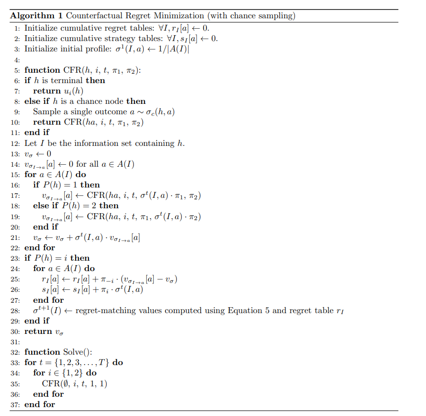Pseudocode for vanilla CFR.

Essentially, you initialize your strategy profile to a random uniform probability of choosing an action for each Information Set.

Then, you can start iterating the algorithm, updating the counterfactual value by self-play, the value updates are propagated through the terminal histories, and weighted by this reach probability (determined by our current strategy).

The strategy profile is then selected proportional the regret using Regret Matching.

Monte-Carlo CFR

With Vanilla CFR, each iteration requires us to traverse an entire game tree since we update ${\sigma }_i^{T+1}(I,a)$ for every single information set $I$ and every action $a$ on each iteration.

However, this is simply too slow with large games such as No-Limit Heads Up Texas Hold’Em Poker. MCCFR can help the speedup convergence to an approximate Nash Equilibrium.

With MCCFR, we avoid traversing the entire game tree on each iteration while still having the immediate counterfactual regrets be unchanged in expectation. We do this by restricting the terminal histories that we consider on each iteration.

Let $Q=\{Q_1,\dots ,Q_r\}$ be a set of subsets of terminal histories $Z$ (i.e. $Q_j\subseteq Z$), such that their union spans the set $Z$ (i.e. ($Q_1\cup \cdots \cup Q_r)=Z$.

Each of these subsets is called a block $Q_j$.

On each iteration, we will sample one of these blocks and only consider that block. Let $q_j>0$ be the probability of considering $Q_j$ for the current iterations (where ${\sum }_{j=1}^r{q}_j=1$).

The probability $q(z)$ of considering terminal history $z$ on the current iteration is given by $q(z)={\sum }_{j:z\in Q_j}{q}_j$ Then, the sampled counterfactual value when updating block $j$ is $\tilde{v}(\sigma ,I|j)={\sum }_{z\in Z_I\cap Q_j}\frac{1}{q(z)}{u}_i(z){\pi }_{-i}^{\sigma }(z[I]){\pi }^{\sigma }(z[I],z)$

The paper proves that the expectations of the sampled counterfactual value is equal to the counterfactual value ${\mathbb{E}}_{j\sim q_j}[\tilde{v}(\sigma ,I|j)]=v_i(\sigma ,I)$

So in the immediate counterfactual regret, we can use the following $R_{i,imm}^T(I,a)=\frac{1}{T}{\sum }_{t=1}^T({\tilde{v}}_i({\sigma }_{(I\to a)}^t,I)-{\tilde{v}}_i({\sigma }^t,I))$

Note to self

I am still having trouble going from the math equations to a full on algorithm that does this.

There is also a speedup to this that I am not aware about.

Old notes

Explanation of notations:

• $\sigma$ is a strategy profile which consists of a strategy ${\sigma }_i$ for each player $i$
  • ${\sigma }_i^t$ is the strategy for player $i$ at time $t$ (assigns probability distributions over $A(I)$)
• $A$ is the set of all game actions
• $I$ is an Information Set
  • The is the information that a player can see. Distinction between State and Set
• $A(I)$ is the set of legal actions for information set $I$
• History $h$ is the sequence of actions from the root of the game
• ${\pi }^{\sigma }(h)$ is the reach probability of history $h$ if all players choose to play according to strategy $\sigma$
  • This is where “chance sampling” comes into play, because we consider reach probabilities to more efficiently train our algorithm

More notation:

• $Z$ denotes the set of all terminal game histories (sequences from root to leaf)

• $u_i(z)$ is the utility of player $i$ at terminal history $z\in Z$

• The counterfactual value at non-terminal history $h$ is $v_i(\sigma ,h)={\sum }_{z\in Z,h⊏z}{\pi }_{-i}^{\sigma }(h){\pi }_i^{\sigma }(h,z)u_i(z)$

We use counterfactual values to update counterfactual regrets.

The counterfactual regret of not acting action $a$ at history $h$ is $r(h,a)=v_i({\sigma }_{I\to a},h)-v_i(\sigma ,h)$

• where ${\sigma }_{I\to a}$ is the profile $\sigma$ except that at $I$, action $a$ is always taken

The counterfactual regret of not taking action $a$ at information set $I$ is just the sum of histories, so $r(I,a)=\sum _{h\in I}r(h,a)$

• You know the counterfactual values since this is a self-play algorithm
• $r_i^t(I,a)$ is the regret of player $i$ at time $t$ for not taking action $a$ at information set $I$ (measures how much player $i$ would rather play action $a$ at information set $I$)
• The cumulative counterfactual regret is $R_i^T(I,a)={\sum }_{t=1}^T{r}_i^t(I,a)$

We use the cumulative counterfactual regret to update the current strategy profile via Regret Matching: ${\sigma }_i^{T+1}(I,a)=\{\begin{array}{ll}\frac{R_i^{T,+}(I,a)}{{\sum }_{a\in A(I)}{R}_i^{T,+}(I,a)}& {\sum }_{a\in A(I)}{R}_i^{T,+}(I,a)>0\\ \frac{1}{|A(I)|}& \text{otherwise}\end{array}$

• where $R_i^{T,+}(I,a)=\max (R_i^T(I,a),0)$

In Games of larger state spaces → For more complex games, where there are quintillions of information sets, this is too large to iterate over for convergence of mixed strategies.

The key idea is that we can approximate information sets, by using imperfect recall. See Game Abstraction

Theoretical Analysis (Regret Bounds)

Notes for me explaining the poker AI

My thoughts: CFR finds the best response to the opponent’s strategy. Over time, this converges to the Nash Equilibrium.

Related Concepts

• Information Set