Value Iteration

I am learning value iteration through two different sets of notations, from David Silver and CS287 by Pieter Abbeel.

It is confusing because value iteration propagates from the terminal states (I guess this is pretty standard, this is how Dynamic Programming works).

Unlike Policy Iteration, there is no explicit policy, and intermediate value functions may not correspond to any policy.

You should first familiarize with Value Function and Optimal Value Function.

Problem: find optimal policy $\pi$ Solution: Iteratively apply the Bellman Equation Optimality Backup: $v_{i+1}(s)=\underset{a}{\max }{\sum }_{s^{\prime },r}p(s^{\prime },r|s,a)(r+\gamma v_i(s^{\prime }))$

• We initialize $v_0(s)=0$ for all states.
• We use $v_i$ to update $v_{i+1}$, therefore we can get $v_1$ from $v_0$.
• Do this for as many time steps as you need. As $i\to \infty$, we see that $v_i$ converges to $v^{\ast }$.

Intuition

#gap-in-knowledge Understand why value iteration works (I understand the algorithm)

Think about this intuitively as a sort of lookahead. The more iterations $i$ you have, the more the values can propagate, and the better the value functions are going to be represent the optimal function, since you are taking the max every time.

Ok, this is still not intuitive to me, see proof below.

Using this Optimal Value Function, we then get an optimal policy $\pi$ $\pi (s)=\underset{a}{\mathrm{argmax}}{\sum }_{s^{\prime },r}p(s^{\prime },r|s,a)(r+\gamma v_k(s^{\prime }))$ The algorithm is described by:

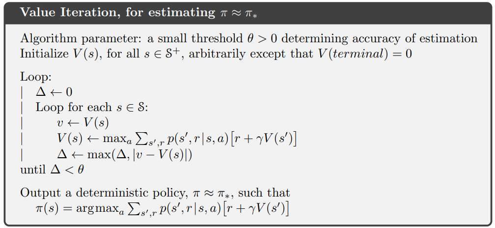
• In here, we generate the policy only at the very end, since the Bellman Optimality Backup does not depend on a policy, we only need to look at the value function. This is not the case for Value Iteration

And so you just build a table and iteratively update the table using Iterative DP. Still need to implement this from scratch, working through it through the homework.

In CS287, a good run through of the grid example is 23:03.

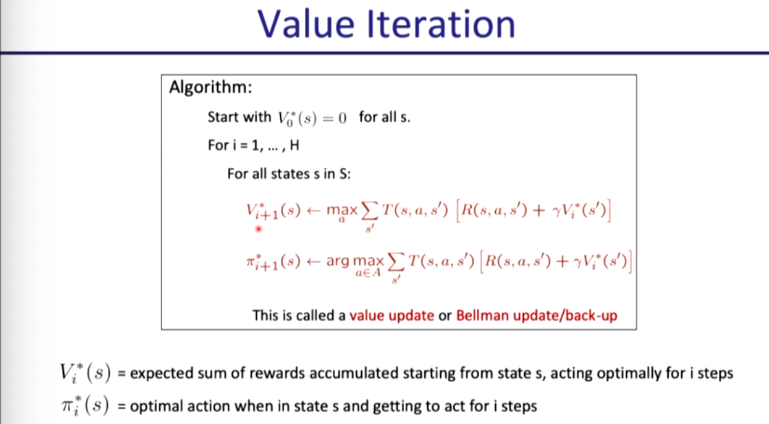
Alternative Notation

This is notation from the CS287 lecture. From an implementation perspective, it makes more sense to use $T(s,a,s^{\prime })$ and $R(s,a,s^{\prime })$ instead of $p(s^{\prime },r|s,a)$ and $r$ because it’s just easier as a vectorized implementation in code.

Value update: $V_{i+1}^{\ast }(s)={\max }_a{\sum }_{s^{\prime }}T(s,a,s^{\prime })[R(s,a,s^{\prime })+\gamma V_i^{\ast }(s^{\prime })]$ And so the optimal policy is just taking the $\text{argmax}$ instead of the $\max$ ${\pi }_{i+1}^{\ast }(s)={\text{argmax}}_a{\sum }_{s^{\prime }}T(s,a,s^{\prime })[R(s,a,s^{\prime })+\gamma V_i^{\ast }(s^{\prime })]$

#todo Convert into LabML notes

Implementation in Python

# Value Iteration, vectorized implementation
for i in range(H):
	v= self.value_fun.get_values()
	next_v = np.max(np.sum(self.transitions * (self.rewards + self.discount * v), axis=2), axis=1) # Bellman Optimality Backup
	self.value_fun.update(next_v) # Update value function
 
	pi_next_idx = np.argmax(np.sum(self.transitions * (self.rewards + self.discount * v), axis=2), axis=1)
	pi = np.zeros(shape=self.policy._policy.shape)
	pi[np.arange(pi.shape[0]), pi_next_idx] = 1
	self.policy.update(pi) # Update policy
 

Intuition / Visualization

Okay, so I did the assignment for value iteration, so on each iteration, the value of the cells propagate backwards. Okay, you need to understand at an implementation level how the value functions and rewards are defined, i.e. Reward Engineering.

So you can see for your rollouts in the assignment, as your iteration $i$ increases, you the cells farther and farther from the reward learn to propagate.

#gap-in-knowledge I still need to build Intuition on this convergence. I know that the algorithm works if I apply it correctly, but now, it’s about getting the proof.

I think maybe the key in understand is this idea of being able to act for $i$ steps, and this is how the values propagate.

Proof of Convergence

The intuition is to show that $V_{t+1}(s)=V_t(s)$ as $t\to \infty$

Geometric Series

Proof 2: Thinking of it as a Contraction, isn’t that the same thing? Fact: The value iteration update is a Gamma Contraction in max-norm.

Corollary: Value iteration converges to a unique fixed point.

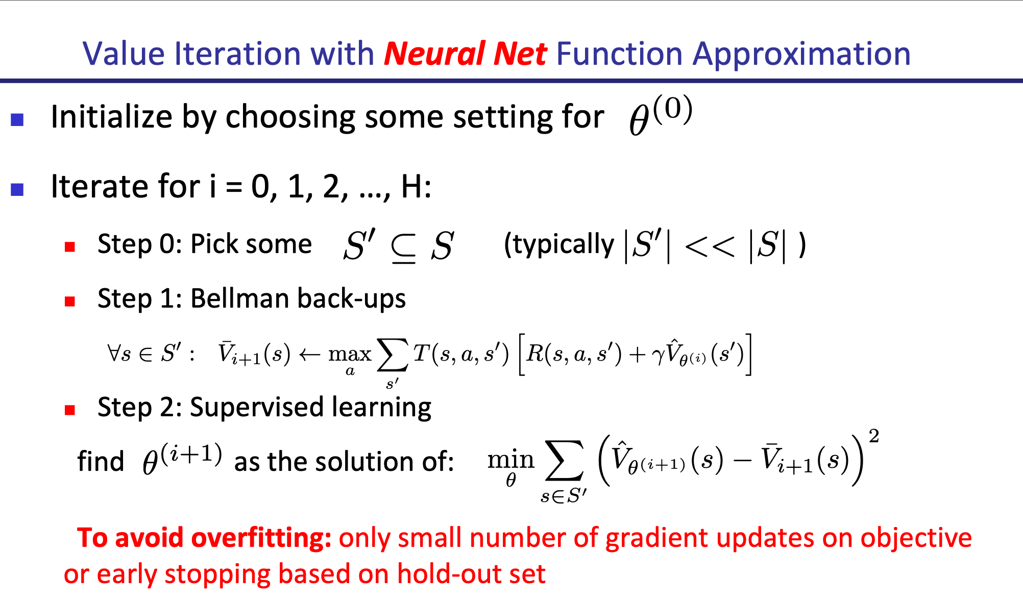
Value Iteration with Value Function Approximation

If there are very large state spaces (or you work in a continuous state space), you can first do Discretization.

Another approach is to do VFA.

For example, you can use a Neural Net.